Tides and their seminal impact on the geology, geography, history, and socio-economics of the Bay of Fundy, eastern Canada
Con Desplanque
27 Harding Avenue, Amherst, NS B4H 2A8
David J. Mossman
Department of Geography, Mount Allison University, 144 Main St., Sackville, NB E4L 1A7
Date received: April 16, 2003 ¶ Date accepted: June 6, 2004
Dedicated to two dear, patient and lovable ladies, Elly and Marie
"Into this Universe, and why not knowing,Nor whence, like water willy-nilly flowing;
And out of it, as wind along the Waste;
I know not whither, willy nilly blowing."
Rubáiyát of Omar Khayyám
Quatrain XXIX
-
Wave And Tide Fundamentals
- Prologue
-
Waves and water particles
- Water waves: vibrations subject to gravity
- Wave forms and wave types
-
Tides and tide generation
- Introduction
- Tide prediction
- The tide-producing forces
-
Variations in strength of the tides
- Gravitational influences and accelerations
- The distance factor
- Springs and neaps
- Diurnal inequality
-
The Coriolis effect
- Overview
- Fundamental relationships
- Applications to tides and water currents
-
Regional tides
- Terms of reference
- Overview of regional tides along the eastern Canadian seaboard
- Graphical synthesis of regional tides
- Additional considerations
- A succession of standing and progressive waves
-
Tides of the North Atlantic
- Water particle movements
- Tidal constituents and harmonic analysis
- Equinoctial tides: east vs west
-
Tides of the Gulf of Maine
- A degenerate amphidromic system
- Sills, banks, and channels
- Tides pre and post-Pleistocene
-
Tides of the Bay of Fundy
- Introduction
- Geologic origin of the Bay and its tides
-
Characteristics of Bay of Fundy Tides
- Resonance and range of modern Fundy tides
- Exponential increase in tidal range and amplitude
- Significance of diurnal inequalities in the Bay
- Tidal cycling at Herring Cove (Fundy National Park)
-
Impacts of Fundy tides
- Erosion
- Sedimentation and related processes
-
Tidal bores in Estuaries
- Tidal volume, tidal prisms
- Waves of translation – tidal bores
- Limiting condition for bore development
- Tidal bores in the Bay of Fundy
- Quiantang River bore, China
-
Ebb and flow in estuaries
- Introduction
-
Reshaping the tidal wave through time
- The Shubenacadie River estuary
- The Cornwallis River estuary
- The Reversing Falls – a unique estuarine feature
- Tidal power
- Prospects for Fundy tidal power
-
Ice phenomena in a Bay of Fundy estuary
- Winter conditions: a short case history
- The phenomenon of ice walls
- Astronomical cycles and ice build-up
- Hazards versus benefits of ice walls
- Ice-related problems in Bay of Fundy estuaries
-
Sea-level changes and tidal marshes
- Postglacial sea-level rise
- Memories of the marshes
- Coastal erosion
- Coastal defence
- Overview of marsh types
- Tidal flooding and marsh growth
- Historical development of the tidal marshes
- Rehabilitation and reclamation
-
Storm tides in the Bay of Fundy
- Introduction
- Atmospheric pressure changes and wind set-up
- The Saxby Tide, 1869: a prediction fulfilled
- Height of the Saxby Tide
- The storm tide of 1759
- The Groundhog Day storm, 1976
-
Periodicity of the tides
- Introduction: The Saros cycle
- Astronomy and the variations of tides
- The largest astronomical tides
- Coincidence of storm tides with Saros
- Probability of a repeat of the Saxby Tide
-
Tidal boundary problems in the coastal zone
- Introduction: caveat emptor!
- Measurement of tidal levels
- Tide prediction: mean sea level and mean high water
- The water's edge: confusion in legislature and literature
- De jure maris
- Boundary issues
- Determination of MHW, Bay of Fundy
- The bottom line
- Conclusions
Preface (TOP)
by Gordon FaderFrom the earliest European exploration of the New World in the 17 th Century, mariners have been acutely aware of the extreme high tides and associated strong currents of the Bay of Fundy. Indeed the region is known internationally for tides that can reach 15 m or more in height and expose vast expanses of seabed during low water. Local tourism actually invites potential visitors to come and walk on the ocean floor. For those who go down to the shoreline, knowledge of the rising tides is an essential survival tool, as in places these tides can literally outrun those who venture too far offshore.
Recent interest and debate in both the Canadian and global press has focused on whether the tides of Fundy are indeed the highest in the world as claimed by many in Atlantic Canada. The title is also claimed by communities in Ungava Bay, northern Quebec. However, recent research by the Canadian Hydrographic Service indicates that the Fundy tides likely outrange those of Ungava Bay by just a few centimetres. But to be fair, the margin of error is greater than the difference, and appropriate data for a meaningful comparison do not exist. Of course, the ultimate question is: why does the Bay of Fundy have such high tides? Surely it can't be just the narrowing shape and shoaling of the bay. And how long have these tides existed: are they a relatively new phenomenon of postglacial emergence? And perhaps more importantly, will the tides change in the future with rising water levels? The development of coastal areas through continued urban sprawl and the maintenance of large areas of dykeland depend on such an understanding.
But there is more to the tides than just an elevational shift of water. These tides drive much of the richness of the Fundy and Gulf of Maine ecosystem through movement of over 100 cubic kilometres of water into the Bay each tidal cycle. Such a massive exchange thoroughly mixes the waters and greatly increases productivity, a process that extends well out into the Gulf of Maine. These nutrient-enhanced fast-moving waters nourish rich fisheries in the Bay and Gulf, particularly with regard to sea scallops, and provide for a substantial sustainable economic return for the region. Recent seabed mapping has discovered large areas of the floor of Fundy covered in unique linear mussel bioherms never before seen on the adjacent Scotian Shelf. Even migrating shorebirds, such as the semipalmated sandpiper, depend on Fundy tides and associated vast mudflats for the provision of essential food to support their long migration from the Canadian North to South America. On the other hand, the Fundy tides result in a cooler climate for the region. For those who live in Nova Scotia's Annapolis Valley, a trip to the Fundy shoreline is a welcomed relief from oppressive summer heat. In contrast, in winter strong westerly winds that blow across the Bay often pick up moisture and produce large local snowfalls ("Fundy flurries") in the Annapolis Valley.
The fast moving waters clocked at over 16 km per hour at Cape Split in the inner Bay of Fundy have also produced dramatic effects on the seabed. Extensive desert-like sand dunes cover many areas, and in Chignecto Bay and Minas Channel constricted areas are scoured down to bedrock in depressions as deep as 60 m. I have always said that if you want to experience the wrath of God, take a hike to Cape Split, a new provincial park at the eastern end of North Mountain, Nova Scotia, and stand at the edge of the 100 m cliff at the time of maximum tidal flood. There you will observe impressive roiling and boiling of the sea, with the generation of large vortices, as the ocean becomes river-like in its inward surge.
Having led many scientific expeditions to study the marine geology of the Bay of Fundy, I am always amazed by the unique and rapidly changing environmental conditions there, and their imprint on the seabed. Once, while we were attempting to run a seismic traverse through Minas Channel at slack water, the CCGS Hudson, although traveling at 5 knots, was actually moving backwards. With expensive gear towed behind the vessel I was very worried and not sure what to do in this circumstance so forged ahead at gear-shattering high speed. As we began to escape the clutches of the high current of the channel just off Cape Split, a large oceanographic gyre located in Scots Bay literally shoved the entire ship to the north in an instant. To top it all off a violent thunderstorm raged while all this was going on.
This synthesis report presents a comprehensive anatomy of the Bay of Fundy and its world-class tides. The work is the result of a long collaboration between Con Desplanque and David Mossman. From the beginnings of postglacial high tide development, perhaps 8000 years ago, the authors describe in detail the many physical factors that play a role in the formation and characteristics of the tides, including the dominant near-resonance length of the Bay of Fundy. The influence of geography, morphology, and gravitational forces of the Sun and Moon, as well as a summary of the geological origin of the Bay and a history of its tides, are all expertly presented. Unique characteristics arising from the high tides, such as tidal bores and reversing falls, are part of the synthesis, as are the age-old dream of electricity generation from Fundy tidal power and the unique conditions of severe winter ice. The ever-present hazard potential from combined high tides and storm surges is evaluated with evidence from the great Saxby tide of 1869 and the Groundhog Day storm of 1976.
This publication is a must for oceanographers and oceano-graphic students who want to understand how geography, geology, and oceanography can combine in unique ways to produce such high tides and energy rich events. Those interested in the history and environment of the region will find the paper of particular interest as the tides play a critical role in defining the characteristics of the coastal zone. Engineers who must develop structures in such a coastal zone will see how humankind has attempted to mitigate the effects of such a dynamic system and what some of the predicted and unpredicted results can be. The tides of Fundy truly play a dominant role in the physical, chemical, and biological processes of the region.
The production of synthesis reports like this is becoming more of a rare event, as the modern applied science approach limits opportunities for such a thorough and integrated study. This publication will indeed serve as a definitive benchmark study of the region with the "World's Highest Tides".
Abstract (TOP)
Tides are an ever-present reality in many coastal regions of the world, and their causes and influence have long been matters of intrigue. In few places do tides play a greater role in the economics and character of a region and its people than around the shores of the Bay of Fundy in eastern Canada. Indeed, the Bay of Fundy presents a wonderful natural laboratory for the study of tides and their effects. However, to understand these phenomena more fully, some large perspectives are called for on the general physics of the tides and their operation on an oceanic scale. The geologic history of the region too provides key insights into how and why the most dramatic tides in the world have come to be in the Bay of Fundy.
Tidal characteristics along the eastern Canadian seaboard result from a combination of diurnal (daily) and semidiurnal (twice daily) tides, the latter mostly dominant. Tidal ranges in the upper Bay of Fundy commonly exceed 15 m, in large part a consequence of tectonic forces that initiated the Bay during the Triassic. The existence and position of the Bay is principally determined by a half-graben, the Fundy Basin, which was established at the onset of the opening of the Atlantic Ocean. Due to the proportions of the Bay of Fundy, differences in tidal range through the Gulf of Maine-Bay of Fundy-Georges Bank system are governed by near resonance with the forcing North Atlantic tides. Although Fundy tide curves are sinusoidal, tide prediction calls for consideration of distinct diurnal inequalities. Overlapping of the cycles of spring and perigean tides every 206 days results in an annual progression of 1.5 months in the periods of especially high tides. Depending on the year, these strong tides can occur at all seasons. The strongest Fundy tides occur when the three elements – anomalistic, synodical, and tropical monthly cycles – peak simultaneously. The closest match occurs at intervals of 18.03 years, a cycle known as the Saros. Tidal movements at Herring Cove, in Fundy National Park, illustrate the annual expected tidal variations.
Vigorous quasi-equilibrium conditions characterize interactions between land and sea in macrotidal regions like the Bay of Fundy. Ephemeral on the scale of geologic time, estuaries progressively infill with sediments as relative sea level rises, forcing fringing salt marshes to grow to successively higher levels. Although closely linked to a regime of tides with large amplitude and strong tidal currents, Fundy salt marshes rarely experience overflow. Established about 1.2 m lower than the highest astronomical tide, only very large tides are able to cover the marshes with a significant depth of water. Peak tides arrive in sets at periods of 7 months, 4.53 years, and 18.03 years. For months on end no tidal flooding of the high marshes occurs. Most salt marshes are raised to the level of the average tide of the 18-year cycle. The exact locations of coastal zone water levels such as mean high water and mean low water is a recurring problem and the subject of much litigation.
Marigrams constructed for selected river estuaries illustrate how the estuarine tidal wave is reshaped over its course, to form bores, and varies in its sediment-carrying and erosional capacity as a result of changing water surface gradients. Changing seasons bring about dramatic changes in the character of the estuaries, especially so as ice conditions develop during the second half of the 206-day cycle when the difference in height between Neap tide and Spring tide is increasing, the optimal time for overflow in any season. Maximum ice hazard, including build-up of "ice walls" in Fundy estuaries, occurs one or two months before perigean and spring tides combine to form the largest tide of the cycle. Although "ice walls" and associated phenomena pose hazards for man-made constructions, important natural purposes are served which need to be considered in coastal development and management schemes. Tides play a major role in erosion and in complex interactions among Fundy physical, biological, and chemical processes. Recent observations on mud flat grain size alterations, over deepening areas of the sea bed, and changes in the benthic community indicate changing environmental conditions in the Bay, caused possibly by increased hydrodynamic energy in the system.
Résumé (TOP)
Les marées constituent une réalité omniprésente dans de nombreuses régions côtières du monde, et leurs causes et leur influence intriguent depuis longtemps. Il existe peu d'endroits où les marées jouent un rôle plus marquant au sein de l'économie et du caractère d'une région et de ses habitats que dans le secteur du rivage de la baie de Fundy, dans l'Est du Canada. La baie de Fundy représente effectivement un merveilleux laboratoire naturel pour l'étude des marées et de leurs effets. Il faut toutefois, pour mieux comprendre ces phénomènes, des perspectives élargies des caractéristiques physiques générales des marées et de leur fonctionnement à l'échelle océanique. Le passé géologique de la région fournit lui aussi des indices précieux sur la façon dont les marées les plus spectaculaires du globe sont apparues dans la baie de Fundy et sur les raisons de leur présence.
Les caractéristiques des marées le long du littoral de l'Est du Canada découlent d'une combinaison de marées diurnes (quotidiennes) et semi-diurnes (biquotidiennes), parmi laquelle ces dernières prédominent principalement. Les amplitudes des marées dans la partie supérieure de la baie de Fundy dépassent communément 15 mètres, en grande partie en raison des forces tectoniques qui ont sculpté la baie au cours du Trias. L'existence et l'emplacement de la baie sont principalement déterminés par un semi-graben, le bassin de Fundy, dont l'établissement remonte au début de l'ouverture de l'océan Atlantique. Vu les proportions de la baie de Fundy, les différences d'amplitude des marées à l'intérieur du système du golfe du Maine, de la baie de Fundy et du Banc Georges sont régies par une quasi-résonance avec les marées de contrainte de l'Atlantique Nord. Même si les courbes des marées de Fundy sont sinusoïdales, les prévisions des marées nécessitent la considération d'inégalités diurnes distinctes. Le chevauchement des cycles des marées de vives-eaux et des marées de périgée tous les 206 jours entraîne une progression annuelle de 1,5 mois des périodes de marées particulièrement élevées. Selon l'année, ces marées de grande envergure peuvent survenir toutes les saisons. Les marées les plus fortes de Fundy apparaissent lorsque les trois éléments – les cycles mensuels anomalistique, synodique et tropique – culminent simultanément. Le jumelage le plus proche survient à des intervalles de 18,3 ans en vertu d'un cycle appelé le cycle Saros. Les mouvements des marées de l'anse Herring dans le parc national Fundy illustrent les variations annuelles des marées anticipées.
Les interactions entre la terre et la mer dans les régions macrotidales comme la baie de Fundy sont caractérisées par des conditions de quasi-équilibre intenses. Des estuaires, éphémères à l'échelle des temps géologiques, se remplissent progressivement de sédiments au fur et à mesure que s'élève le niveau relatif de la mer, ce qui force les marais salés en bordure à passer à des niveaux successivement supérieurs. Même si les marais salés de Fundy sont étroitement liés à un régime de marées de grande amplitude et de courants périodiques puissants, ils débordent rarement. Comme ces marais sont établis à environ 1,2 mètre de moins que les marées astronomiques les plus élevées, seules les très grandes marées peuvent les recouvrir d'une couche d'eau d'une profondeur substantielle. Les marées les plus importantes se présentent en série à des périodes de sept mois, 4,53 ans et 18,03 ans. Aucune inondation des marais élevés due aux marées ne survient pendant des mois et des mois. La majorité des marais salés s'élèvent au niveau moyen du cycle de 18 ans. Les emplacements exacts des niveaux d'eau des zones côtières, comme le niveau moyen des hautes-eaux et le niveau moyen des basses-eaux, ne cessent de poser des problèmes et font l'objet de beaucoup de litiges.
Les courbes de marées établies dans le cas de certains estuaires de rivières illustrent de quelle façon les vagues des marées estuariennes se transforment le long de leur trajet pour former des mascarets et dans quelle mesure varient leur capacité de transport de sédiments et capacité d'érosion par suite des variations des pentes de la ligne d'eau. Les saisons qui se succèdent entraînent des changements spectaculaires du caractère des estuaires, en particulier lorsque des glaces apparaissent au cours de la seconde moitié du cycle de 206 jours, quand la différence de hauteur entre la marée de mortes-eaux et la marée de vives-eaux s'accroît, moment optimal de débordement au cours de n'importe quelle saison. Le danger maximal de glaces, notamment l'apparition de « murs de glace » dans les estuaires de Fundy, survient un ou deux mois avant que les marées de périgée et de vives-eaux se combinent pour former la marée la plus importante du cycle. Même si les « murs de glace » et les phénomènes connexes posent des dangers aux constructions érigées, ils servent des fins naturelles importantes qu'il faut considérer dans les programmes d'aménagement et de mise en valeur des côtes. Les marées jouent un rôle marquant dans l'érosion et dans les interactions complexes au sein des processus physiques, biologiques et chimiques de Fundy. Les observations récentes des modifications des grosseurs des grains des vasières, les secteurs d'approfondissement marqué du plancher océanique et les changements survenus dans la communauté benthique révèlent que les conditions du milieu de la baie changent, possiblement en raison de l'énergie hydrodynamique accrue à l'intérieur du système. [ Traduit par la rédaction]
1. Wave and Tide Fundamentals (TOP)
1.1. PROLOGUE
1 Oceans cover nearly three quarters of planet Earth. Our lives are intimately linked to them and to their tides in diverse ways, most of which we poorly appreciate. Subject to fanciful theories and speculations for thousands of years, tides have long piqued our curiosity. Sir Isaac Newton (1642– 1727) first identified gravitational forces as the prime movers in tide generation. He laid the basis of tidal theory, conceiving an "equilibrium tide" that would apply to ideal conditions of a global ocean. Pierre Simon de Laplace (1749– 1827) shares honours with Newton because he formulated equations of motion for tides on a rotating Earth, and was first to distinguish tidal phenomena according to different types (species) of tides. Laplace perceived the harmonic method of analyzing tides, later elaborated by Lord Kelvin (1824– 1907), inventor of the earliest tide-predicting machine in 1872.
2 Yet despite the ease with which tide tables are now constructed, no one to this day really comprehends how gravitational forces work. Neither has anyone been able to conceive a purely dynamic theory to directly relate tide-generating forces to actual tides (Clancy 1969; LeBlond and Mysak 1978). Laplace recognized that there could be no perfect theory, the chief difficulty being Earth's rotation. He preferred to write in terms of tidal waves, with the same periods as those induced by rhythmical components of gravitational forces. The problem of tides is that of a fluid motion modified by the geometry (including depth) of ocean basins, by friction, and by such forces as the Coriolis effect due to Earth's rotation.
3 The ebb and flow of tides provide fascinating measures of an ocean's pulse (Defant 1958). Nowhere does this beat more impressively than in the Bay of Fundy on the western shore of the North Atlantic Ocean. Here the tide attains world record levels, with tidal range approaching 16 m at times of particular astronomical conditions. Storm surges, tidal bores that gain height in an estuary, and great waves that batter the shore: all stir the blood and instil respect for the raw power of nature.
4 Other processes related to tides, among them currents, shifting sediments, erosion, development of tidal estuaries, and salt marsh growth and decay, work more subtly, creating changes over decades, centuries and millennia, rather than in a matter of hours or days. These processes, in turn, evolve in response to postglacial sea-level recovery. The unmistakable hand of Homo sapiens too, is now everywhere evident along the shore, for it is in the world's coastal zones that humankind has by choice become most concentrated.
5 The main purpose of this review is to provide a general survey of tides and an overview of their relationship to, and effect on, the Bay of Fundy (henceforth sometimes referred to as "the Bay"), home to the world's highest tides. Worldwide there is now an increased focus on understanding tidal processes and documenting changes on short-, medium-, and long-term time scales by various historical and scientific means. The Bay of Fundy and its tidal processes form a dynamic entity, and serve as a model for comparison with similar tidal regimes elsewhere.
1.2. WAVES AND WATER PARTICLES
1.2.1. Water waves: vibrations subject to gravity
6 Long before Aristotle (384– 322 B.C.E.) wrote about the relationship between wind and waves, mankind had been engaged in the study of waves. Yet despite the writings of Aristotle, Newton, Kelvin, Stokes, Helmholtz, and others, details of the physics of wave oscillations are still being worked out. Here we no more than touch on this vast subject. Splendid comprehensive elementary treatment of waves – tidal and otherwise – is provided by Pethick (1984), Pugh (1987) and Sverdrup et al (2003).
7 Waves in general play an important role in meteorological and oceanographic processes such as mixing in the upper ocean layer and production of oscillatory currents, as well as a number of processes involving air-water interactions. Ocean waters do not conform precisely to the dynamics of idealized fluids upon which mathematical models of wave behaviour are based. Even so, a water wave is essentially a vibration subject to gravity. With this in mind we briefly examine the birth of waves in water and the characteristic oscillatory behaviour required to produce ordinary tide waves (or "tidal waves", not to be confused with the improper popular synonym for tsunami).
8 In any material at rest, except of course for vibrations on an atomic scale, none of the particles of the material are moving in relation to each other. However when an external force moves some of the particles out of their rest positions without breaking a bond, tension is built up within the material. If the external force is relaxed, the displaced particles will return toward their former positions: to do so they have to move with a certain velocity thus giving them momentum. However, this momentum will not immediately disappear when the particles reach their rest positions. They will overshoot, building up a new tension in reversed direction. The particles will continue to oscillate about their rest positions, their displacement dependent upon the strength of the initial force. Because the moving particles come into contact with other particles that do not move in the same direction or at the same rate, the energy that started the oscillation will eventually be dissipated over more and more smaller, sub-atomic particles, increasing the temperature of the material.
9 At Earth's surface, gravity compels all particles making up a body of water to be collectively drawn as close to the centre the Earth as the container will allow. Hence, the surface area of a small body of water is virtually a flat plane, with all points on it being the same distance from the centre of the Earth. Disturbances from external sources of energy cause some of these particles to move horizontally. The result is that some particles are raised to an elevation higher than the rest plane, leaving a void where they have been removed. When external energy sources are removed, higher particles will tend to move back towards the void, creating an oscillating motion. Another factor that needs to be considered is surface tension. Water particles have an affinity for each other, and when this linkage is disturbed, surface tension will tend to restore the displaced particles to their original positions. However surface tension is a much smaller force than that of gravity, especially if large masses are involved, and it is only important when the displacements are small.
10 When displacement occurs, more water particles per unit area are above a certain datum plane in a given area than there are at nearby unit areas. (Since water is about as compressible as high strength steel, this means that the water level in the area where the particles are moved is higher than the original rest plane.) In this highly simplified wave, the place where the water is at the highest level is called the crest and that of the lowest level is called the trough.
11 To illustrate some further basic concepts, imagine a stone thrown into water: the stone's impact causes a set of concentric ripples to move outward. The distance between the crests of two subsequent ripples is called the wave length, L. The time it takes for a wave to move over the distance of one wave length is called a period or cycle, T. The vertical distance between the crest (High Water) and the trough (Low Water) is the height, or range of the wave. Half the range is called the amplitude A, and represents the maximum displacement of the wave from the rest plane. The frequency, f, is the number of cycles that pass a given location during a unit of time. The most common period of a tidal wave is 12.42 hours; thus its frequency (the reciprocal of the period) is 0.08051 cycles per hour. The wave speed or celerity, c, is the horizontal rate of advance of the wave as a whole, where c = L/t = f · L (see Fig. 1.).
Fig. 1 Characteristics of wave generation, shape, and propagation given for degrees and radians, where Ht is the shape of the wave as a function of time t, Hx is the shape of the wave as a function of distance x, n is the angular speed of the wave in radians, and K is the wave number.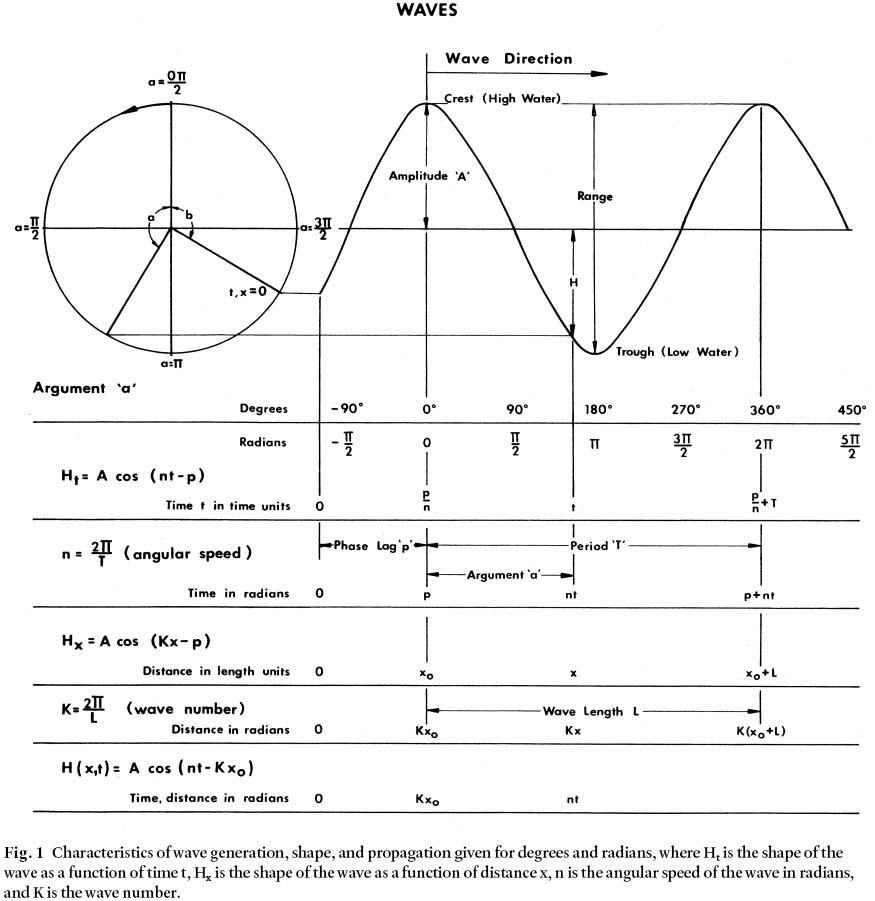
1.2.2. Wave forms and wave types
12 The form of a water wave is most commonly like a sine or cosine curve. As the crest of a wave is its most visible feature, it is customary to express the shape of a wave as a function of time t:


13 These equations describe a progressive wave moving in a positive x-direction at the distance x in time t. When the argument (n · t – k · x) is equal to zero, High Water will occur. This means that High Water will occur when t = T · x/L = k · x/n.
14 When the wave moves in the opposite (negative) x-direction, the appropriate equation becomes:

15 When two waves with the same amplitude A, and the same frequency f or period T, are moving in opposite directions, the resultant wave will be a standing wave which can be described by the following equation:

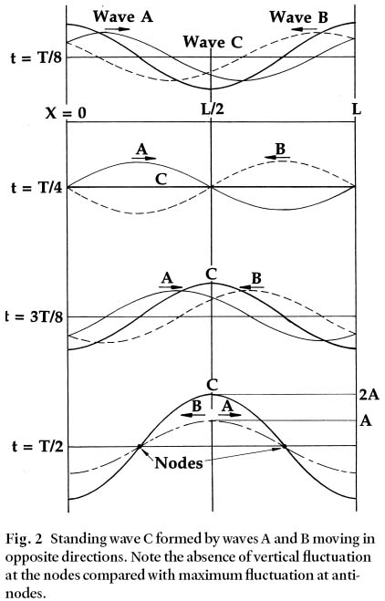
16 Figure 2 illustrates the consequences of such an event. Hs is maximum when t = 0, or t = T and x = 0, or x = L or when t = 0.5T and x = 0.5L. Hs is minimum when t = 0.5T and x = 0 or x = L (or when t = 0, T and x = 0.5L). Hs is 0 at all places when t = 0.25T or t = 0.75T or at all times when x = 0.25L or x = 0.75L (node). Note that at any value of t the shape of the wave will be that of a cosine curve. At the closed end of a channel, should a progressive wave be reflected, a standing wave may form. Thereby the energy of the wave is temporarily transformed into potential energy. In theory wave height can double as indicated by the factor 2A in (6). The maximum vertical fluctuations occur at the end of the channel and at locations that are distant from the end by multiples of half the wave length. These locations are called "anti-nodes", whereas at the "nodes" halfway between there will be no surface fluctuations. However, strong currents will be in evidence because the water flows to and fro between the anti-nodes. Consequently, when the water surface is high at the "even" anti-nodes, it will be low at the "odd" anti-nodes.
Fig. 2 Standing wave C formed by waves A and B moving in opposite directions. Note the absence of vertical fluctuation at the nodes compared with maximum fluctuation at anti-nodes.
Display large image of Figure 2
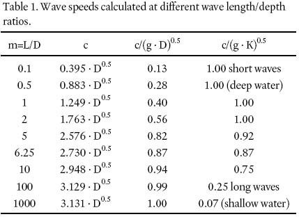
17 In the foregoing discussion, it is assumed that the wave height is small relative to wavelength and water depth. Although the range of the wave will always be small relative to wave length, it need not be so with respect to the depth. As derived from the dispersion relation, the wave speed of a sinusoidal wave in a body of water can be expressed as:

Table 1. Wave speeds calculated at different wave length/depth ratios.
Display large image of Table 1
18 In the Atlantic ocean, where water depths are in the order of 5000 metres and both the distance across and the tidal wave length, L, are about 5000 km, the value of m is approximately 1000. Thus, even oceanic tidal waves are shallow water waves, affected by ocean depth. Particle motions in shallow waves are uniform with depth. Since water depth affects celerity or wave speed, waves moving into shallower water will decelerate. If, at the right flank of the wave, water is shallower than on the left flank, the wave on the right side will fall behind the wave crest on the left side. In effect, wave crests tend to conform to the depth contours over which they are moving. Thus, a wave approaching an island that rises very steeply from the ocean bottom, will pass the island unchanged, whereas a wave approaching an island surrounded with a gradually shallowing shelf tends to move toward the shore line in nearly concentric circles. This bending of the wave crest because of changing depths is called refraction.
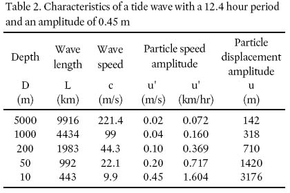
19 There is a relationship between the wave speed, c, and the speed of the particles in the oscillating body of water. The particle displacement amplitude, u', can be expressed as follows:


Table 2. Characteristics of a tide wave with a 12.4 hour period and an amplitude of 0.45 m
Display large image of Table 2
20 Note that in waters 5000 m deep, particle displacement from its rest position needs to be only 142 m during a tidal period in order to make a tidal wave possible. For shallower water on the continental shelf, the required displacement becomes thousands of metres. The gravitational influences of the Moon and the Sun countering those of the Earth cause these particles to move. In contrast to wind movements, which only create a shear force at the surface of the water body, these gravitational influences act on particles at all depths of the ocean.
21 We turn next to the generation of shallow-water waves in the oceans.
1.3. TIDES AND TIDE GENERATION
1.3.1. Introduction
22 Tides, the longest of oceanic waves, involve alternating rise and fall of sea level due to gravitational effects exerted on the Earth by the Moon and Sun. People have long recognized that there is a connection between tides and the positions of the Moon and Sun relative to Earth. However, the nature of this connection is by no means obvious, and the influence of these celestial bodies on tidal events results in complex flow patterns. Nevertheless, the magnitude of the effects that generate tides can be precisely calculated from the astronomy alone, the chief caveat being that the ocean's response to these effects will be constrained by continental landmasses, the Earth's rotation, the geometry of ocean basins, and the transience of weather. According to Newton's equilibrium tidal theory, an ideal wave forms instantaneously upon an Earth uniformly covered by a deep layer of water, under the influence of the gravitational effects of the Moon and Sun. This theory is not meant to provide a realistic picture of what actually occurs in nature, but it does give accurately the tidal periods, the relative forcing magnitudes, and the astronomical phases of the tides. It is this idealized calculation that forms the cornerstone upon which tidal analysis and predictions are based.
23 The dynamic tidal theory employed by oceanographers shows that there is no wave crest formed instantaneously in the ocean directly under the Moon (or Sun), or at its antipodal point. The vertical tide movements at most locations can be represented by a time-space graph in the form of a modified sinusoidal curve like that of a simple harmonic motion. In harmonic motion, an object is accelerated by a variable force, the strength of which can be represented by a sine curve. Half the time this force will have a positive direction. When this force becomes zero at the moment it changes to a negative direction, the resulting velocity will reach its maximum strength. The velocity graph throughout the cycle will also be sinusoidal, but 90° out of phase with acceleration. The object moved by the force will reach its farthest displacement in the positive direction when velocity becomes zero. This means that instead of a "tidal bulge" as customarily shown to be formed beneath the Moon, there will be a depression. Thus, generally only horizontal or "tractive" forces are responsible for generating tidal movements in the ocean.
24 It is important to note here the three main astronomical reasons for variations in the strength of these gravitational forces:
- Variable distance between Moon and Earth. This variation causes the greatest deviations from the average (mean) tide in the Bay of Fundy. Because the Moon's orbit is elliptical, once a month at perigee the Moon is closest to the Earth, and thus its gravitational pull is then at its greatest, resulting in stronger than average tides. These so-called perigean tides recur every anomalistic month of 27.555 days.
- Variable celestial positions of the Moon, Sun, and Earth relative to each other. The cycle of the Moon's phases in which there are two sets each of spring and neap tides, is the synodical month of 29.531 days. In the first set, spring tides are stronger than average because the Earth is either between the Sun and Moon (full moon), or the Moon is between Earth and Sun (new moon). A week later, during the first or last quarter of the moon, its gravitational influence is diminished by that of the Sun, which is then acting at right angles. The resulting tides, weaker than usual, are called neap tides.
- Declination of the Moon and Sun relative to the Earth's equator. Declination is the angular distance in degrees between a heavenly body and the celestial equator (the plane in which the Earth's equator is situated) when it passes through the local meridian. A complete cycle, in which the Moon crosses the Equator twice, lasts 27.322 days and is called a tropical month. However, it takes 18.6 years for the Moon to complete its cycle of maximum declination, ranging between 28.5° N and 28.5° S with reference to Earth's equatorial plane.
25 One can expect stronger than usual tides a few days later than full and new moon, and weaker tides near the quarter phases of the moon. There is a certain inertia in the development of the tides, analogous to the fact that the months of July and August are on average warmer in the Northern Hemisphere than June, when the days are longer and the Sun is higher. For this reason the highest tides occur a few days after the astronomical configurations which induce them.
1.3.2. Tidal prediction
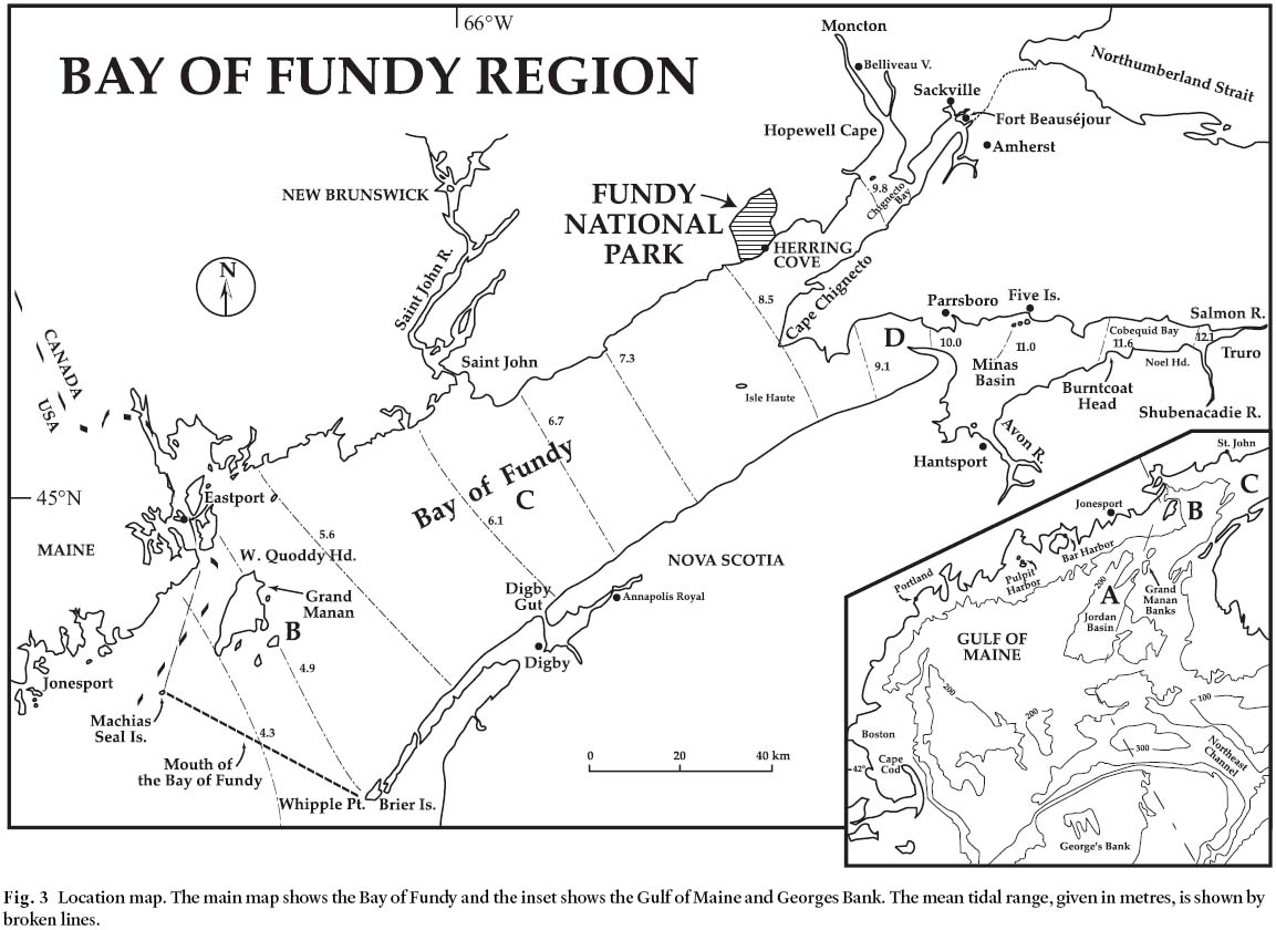
26 Tidal predictions are based on harmonic analysis of local tides. In the Bay of Fundy (Fig. 3) the principal hydrographic station is located at Saint John, New Brunswick. [Henceforth, New Brunswick will be abbreviated to N.B. and Nova Scotia to N.S.] Predictions are made and published annually for this reference port. Upon analysis, the observed tides are broken down into a large number of cosine curves, so-called tidal constituents, each representing the influence of a particular tidal influence or characteristic of the local tide. The first seven harmonic constituents listed in Table 3 account for >90% of the total variability of the tides. As many as 62 tidal constituents are routinely used for tide prediction. The M2 constituent represents the influence that the Moon has on the local tides, supposing for simplicity that it makes a circular orbit around the Earth in the plane of its equator at a distance resulting in (most cases) average tides. The S2 constituent represents the Sun's gravitational influence, assuming that Earth moves in a circular orbit around the Sun at a distance producing the average effect, and assuming that the Earth's equator is located in the ecliptic. Other constituents make corrections to these basic assumptions, because of variations in actual and sometimes apparent movements of these heavenly bodies. Constituents with the subscript "2" repeat themselves twice a day, causing two daily (semidiurnal) tides. Those with subscript "1" occur once a day, and those with subscript "4", four times a day. The K4 constituent is the main overtide in the Bay of Fundy. It appears where the usual sinusoidal shape of the tidal wave is distorted upon entering shallow, narrowing inlets. This process results in loss of symmetry of the tidal wave, causing the water to rise faster than it will drop in the following ebb (Forester 1983; Canadian Hydrographic Service 1981).
Fig. 3 Location map. The main map shows the Bay of Fundy and the inset shows the Gulf of Maine and Georges Bank. The mean tidal range, given in metres, is shown by broken lines.
Display large image of Figure 3
Table 3. Constituents in the Gulf of Maine - Bay of Fundy - Georges Bank system (in metres)

Display large image of Table 3
27 Nowhere does the pulsating ebb and flow of the tide beat more impressively than in the Bay of Fundy (Defant 1958). Here the tidal range exceeds 16 m at times of particular astronomical conditions. Fundy tides are an integral part of the semidiurnal tidal system prevailing in the North Atlantic area (Davis and Browne 1996).
1.3.3. The tide-producing forces
28 In Atlantic Canada there are usually two unequal tides each day. They are due to the combined gravitational effects of the Moon and Sun, and the centrifugal forces resulting from the revolution of the Earth-Moon and Earth-Sun systems around their common centres of gravity. For instance, the Earth and the Moon revolve in essentially circular orbits round their combined centre of mass (barycentre) every 27.3 days (sidereal month). Thus every point on Earth has an angular velocity of 2π per 27.3 days, and each will experience an equal acceleration as a centrifugal force away from the Moon. The total of all these forces on the mass of the Earth is balanced by the total gravitational effects of the Moon's mass on Earth's mass, keeping the Earth on its orbit, just as the gravitational effects of the Earth keep the Moon on its orbit (Doodson and Warburg 1941; OPEN 1993). The magnitude of the force (Fg) keeping these bodies on their respective orbits can be expressed with the following equation:

29 The magnitude of FTP (Fig. 4) on a particle with the mass m at point Q, in relation to a similar particle at the centre of the Earth, for example (given the Earth's radius = a), is:


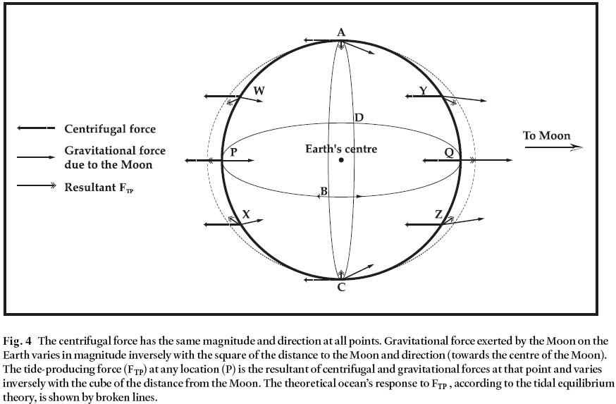
Display large image of Figure 4
30 These forces will cause particles in the oceans to move along looping paths of limited distances, but enough to cause the tidal movements. The looping patterns are thus variable for each latitude, season, and phase of the Moon – see Desplanque and Mossman (1998a) for charts of particle movements. For example, during its new- and full-moon phases, the Moon makes its transit through the local meridian at 12:00 and 24:00 hours, and during its first and last quarter phases at 06:00 and 18:00 hours. Individual water particles reach their most westerly displacement position during the evening in the summer, and during the morning in the winter and, whereas the tides in the ocean are chiefly semidiurnal, the looping tracks of the individual particles are mainly diurnal. The ocean water would thus receive an impulse with every second oscillation, in contrast to the pendulum of a grandfather clock that, through its escapement wheel, receives an impulse every oscillation. The dimensions of the loops indicate that the movement of the water particles can maintain the tidal movement in deeper waters, but not in shallow ones. The movements, in sum constituting a progressive tidal wave, measure in mid-ocean a few hundred metres at most. However, like water spilled from the edge of a shallow dish, tidal effects become more evident in shallowing coastal waters where rotary tidal currents of amphidromic systems are impeded.
1.3.4. Variations in strength of the tides
1.3.4.1. Gravitational influences and accelerations.
31 On average, the Earth requires 24 hours to revolve with respect to the Sun. Similarly the Moon seems to travel around the Earth in 24 lunar hours, equivalent to 24.84 solar hours. To illustrate the different possible situations, the Sun is used in the following discussion; the Moon could also be used, but the periods would then be measured in lunar hours.
32 First, consider the Sun's gravitational influences on a particle of water subject to semidiurnal oscillations near the Equator. At sunrise, around 06:00 hours, the particle is on (terminator) circle T. It is not accelerated horizontally (Fig. 5). However, shortly afterwards it will be drawn toward the east, to be accelerated strongest in that direction at 09:00 hours. The acceleration ceases at noon, to be replaced shortly afterwards by a westerly acceleration, which will be at its maximum at 15:00 hours. At 18:00 hours this acceleration will be reversed to an easterly acceleration. The process is repeated over and over again in cycles of 12 solar hours. When the acceleration in an easterly direction stops at 12:00 hours and at 24:00 hours, the particle affected by it will reach its maximum velocity in this direction. The maximum velocity in a westerly direction will occur at 06:00 and 18:00 hours (Fig. 5). The particle will not move at 03:00, 09:00, 15:00 and 21:00 hours. Note that when the particle is accelerated the fastest to the east, it is at its most westerly position in its semidiurnal oscillation.
33 If the vertical accelerations caused by the Sun and Moon were of any consequence, the same reasoning could be used. In the case of the Sun these accelerations would be strongest upward at noon and midnight, and strongest downward at 06:00 and 18:00 hours. This means that the displacement of the water surface (Fig. 5) would be downward at noon and midnight.
Fig. 5 Development of the semidiurnal oscillation is shown by the relationship between acceleration, velocity, and displacements of water particles (in E-W direction in left column, N-S direction in right column) resulting from gravitational influences of the Sun and Moon on Earth. (The Coriolis effect is not taken into consideration here.)

Display large image of Figure 5
34 Because the horizontal or tractive accelerations need not compete with much stronger terrestrial gravitation, they can set water particles in motion in the almost frictionless ocean because neighbouring particles are subject to almost identical influences. A constant acceleration of 8.4 · 10 8 · g (8.237 · 10 -7ms -2, applied for one hour to a particle originally at rest, will impart to that particle a speed of 0.003 ms -1, or 10.8 m/hr. The distance travelled in that interval is 5.4 m. In a three hour period, the velocity will have been 24.4 m/hr and the distance travelled 48.6 m.
1.3.4.2. The distance factor.
35 Once in the anomalistic month of 27.555 days, the Moon's distance from Earth is 92.7% of the mean distance between the two bodies. Since the effect of the Moon's gravitation on the particles in the ocean is inversely proportional to the cube of the distance, the effect is 1.255 times stronger than the average effect. Approximately 14 days later, with the Moon in apogee, the distance is 1.058 times the average distance and the Moon's effect is reduced to 84.4% of its average value. The Earth is closest to the Sun shortly after New Year, making its influence 5.2% stronger than average, while in the first days of July its effect is reduced by 4.9%. Thus, in theory, the Moon's effect varies between 0.844 and 1.255 times its average effect because of varying distance, while for the same reason the Sun's effect varies between 0.438 and 0.484 times the Moon's average effect.
1.3.4.3. Springs and neaps.
36 The relationship between synodical month and the mean semidiurnal reappearance of the tide "M2" is given by M2 = 12 (1– 1/M) = 12.42 hours (12 hours and 25 minutes). Twice during the synodical month, the Earth, Moon, and Sun are almost aligned. The gravitational effects of Sun and Moon are additive and the so-called spring tides are stronger than usual. Due to inertia in the development of tides, the highest tides occur a few days after the appropriate astronomical configurations. Such tides are called spring tides because they spring or reach higher than normal. When the tides along the European coastlines are analyzed it turns out that the actual effect of the Sun is between 0.3 and 0.4 times that of the Moon's effect, a little less than the theoretical value of 0.46. Thus, the bimonthly variation in this region is between 0.6 and 1.4 times the mean tide, more than caused by the variation in the distance between Earth and Moon. Small wonder, therefore, that western Europeans have regarded the cycle associated with changing Moon phases as the most important one. When the Moon is in either the first or last quarter, the actions of the Moon and Sun are perpendicular to each other and tend to counteract each other. Because the Moon's effect is the strongest, it will prevail, but in a reduced fashion. When this condition exists, the tides are called neap tides, a Saxon term related to the Germanic word "knippen", to pinch, meaning that they are reduced in size. In waters bordering most of North America, the influence of the Sun on the tides is itself rather "nipped". Consequently, the tidal variations caused by once-monthly so-called perigean tides are much more prominent.
1.3.4.4. Diurnal inequality.
37 Tides are generally semidiurnal, i.e., there are two High Waters and two Low Waters during a day, be it a solar or a lunar day. The strength of tides is modified by changing distances between Earth and Moon, and between Earth and Sun, and also because the Moon and the Sun act from varying directions. Changing declinations of the Sun and the Moon with respect to the plane of the ecliptic cause diurnal variations in the strength of the tides, a phenomenon called diurnal inequality. Usually, both the two High Waters and the two Low Waters during a day are affected, their respective levels being unequal. Elsewhere, High Waters during a day reach almost equal levels, in contrast to the levels of the Low Waters, which may be different.
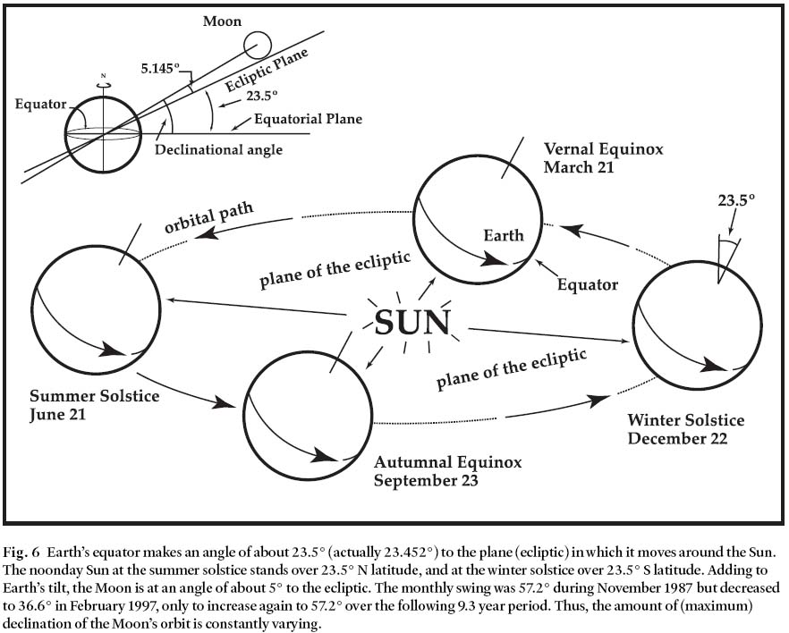
38 The declination of the Sun is due to the fact that the plane of the Earth's equator makes an angle of 23.452° with the plane in which the Earth orbits the Sun (Fig. 6). Hence the Sun appears higher in the sky during summer in the Northern Hemisphere, reaching its highest point at noon on 21 June. Conversely, at noon on 21 December the Sun appears 46.9° lower above the horizon. Thus, summer days are longer than summer nights, and winter days are shorter than winter nights. At an equinox, the Sun is overhead at the Equator on about 21 March and 23 September, the day length is the same as night length everywhere on Earth. The Sun is said to have a north declination between the spring and fall equinoxes, and a south declination during the remainder of the year.
Fig. 6 Earth's equator makes an angle of about 23.5° (actually 23.452°) to the plane (ecliptic) in which it moves around the Sun. The noonday Sun at the summer solstice stands over 23.5° N latitude, and at the winter solstice over 23.5° S latitude. Adding to Earth's tilt, the Moon is at an angle of about 5° to the ecliptic. The monthly swing was 57.2° during November 1987 but decreased to 36.6° in February 1997, only to increase again to 57.2° over the following 9.3 year period. Thus, the amount of (maximum) declination of the Moon's orbit is constantly varying.
Display large image of Figure 6
39 The Moon goes through a similar but much shorter declinational cycle, lasting 27.322 days. As the Moon's plane makes an angle of 5.145° with the ecliptic, the declination of the Moon is more variable than that of the Sun. Thus, there are years when the declination of the Moon ranges from 28.597° North to 28.597° South, 14 days later. This condition existed in 1987 and will occur again in 2005, 18.6 years later. But in 1996 the maximum variation in declination of the Moon ranged between 18.307° North and South.
40 The declinations of the Moon and Sun have a great influence on the directions of the accelerations affecting particles in the oceans. During an equinox, not only days and nights are of equal duration, but the two tides caused by the Sun will also have the same strength. Nor is the Moon able to produce diurnal inequality when it crosses the plane of the Earth's equator. Because the Moon's orbit is never more than 5° from the ecliptic, the Moon's declination is close to the Sun's declination when there is a new moon. At full moon, it has an opposite declination to that of the Sun. Consequently, the only periods during which both Sun and Moon can cause little or no diurnal inequality are when there is a full or new moon near an equinox. These two periods fall annually between 8 March and 3 April, and between 10 September and 6 October. For the remainder of the year either the Moon or the Sun, or both, will be in declination. The role of diurnal inequalities in the Bay of Fundy is explored in greater detail in a later section (5.3.3).
1.4. THE CORIOLIS EFFECT
1.4.1. Overview
41 As a result of Earth's rotation, any object freely moving near or in contact with its surface will veer to the right in the Northern Hemisphere and to the left in the Southern Hemisphere. This is called the Coriolis effect. It affects winds everywhere, and in the oceans it results in the circular motion of water. The French mathematician Gaspard Gustave de Coriolis explained the phenomenon, applicable to frictionless motion, early in the 1800s. The effect is caused by Earth's eastward rotation. At the Equator the eastward movement of the planet's surface is about 1670 km/hr (actually, 6378.16 km · π · 2 /24 = 1669.8 km/hr), but falls off at higher latitudes as the circumference of the Earth, in the axial plane normal to Earth's axis, gradually decreases (OPEN 1993). Thus at 45° latitude the velocity is about 1200 km/hr (1179 km/hr), falling off to zero at the poles. Any object freely moving away from the Equator, north or south, is moved to the east at higher latitudes because of higher eastward inertia. Conversely, an object approaching the Equator from north or south is effectively retarded due to smaller eastward inertia; it is moved to the west as it approaches the Equator from either north or south. Consequently, essentially frictionless objects such as wind and ocean currents, and tidal waters entering and leaving coastal embayments, are deflected to the right in the Northern Hemisphere and to the left in the Southern Hemisphere.
42 In the case of the atmosphere, air moves from high pressure areas to depressions. The depressions are filled from all sides, and air currents are deflected to the right by the Coriolis effect. However, the result is that the winds approaching and converging near the depression, in the Northern Hemisphere, form a cyclonic anticlockwise circulation. Water surfaces beneath a developing atmospheric depression, rise in elevation, drawing water from areas under high pressure systems. Famous whirlpools, such as the Maelstrom off Norway, and the Old Sow near Deer Island in Passamaquoddy Bay in the Bay of Fundy, are also subject to the Coriolis effect.
43 Flat rotating objects such as a record player or merry-go-round can be used to illustrate the Coriolis effect. In terms of vector algebra, the fundamental relations are briefly set out below; they apply to the apparent centrifugal force working on a particle in a circular orbit and its counterpart, the centripetal force, which keeps it on this orbit.
1.4.2. Fundamental relationships
44 In relation to the stars, the Earth rotates once in a so-called sidereal day, which lasts 86 186 seconds. Thus each particle in or on Earth has an angular velocity of w = 2 π /86186 = 7.29 · 10 -5 radians per second. Its linear velocity depends on its distance from the Earth's axis, which runs from pole to pole (Doodson and Warburg 1941).
45 Now consider an object of mass m, moving along the circular path (Fig. 7a) with a velocity V. If it takes t seconds to go around the circle at a constant speed, the object's velocity will be V = 2 π · R/t, in which case the angular speed is w radians per second (w = 2π/t). Thus, the linear velocity V = w · R. If this mass moves from point A to point B on its circular path, it is deflected the distance DB (= x) from the straight path it would have taken had it not been constrained by some force. If the distance AB was covered in t seconds, the force f must have been 2x/t 2 ms -2, because


46 Suppose now that a particle with mass m, is moving along a circle with radius R, at latitude l. Its velocity is R · w, and the centrifugal force acting upon it will be m · R · w 2. Relative to the Earth, it seems to be at rest. However, if it is given a velocity V in the direction of rotation, its real velocity in space will be R · w +V, or R(w + V/R), its angular velocity having been changed from w to (w + V/R), and the apparent centrifugal force acting upon it m · R (w + V/R) 2, which is equivalent to:

47 The first term in (16) is the normal centrifugal force resulting in the equatorial bulge, and is balanced by the slope from Equator to the poles of the Earth. The third term is very small because of the divisor R, and can be ignored. The remaining middle term can be split into vertical and horizontal components (Fig. 7d). The vertical one will affect the local apparent gravity force, but the horizontal component will cause a tractive force acting along the Earth's surface, effectively moving the mass to the right (in this case toward the Equator, the initial motion having been west to east in the Northern Hemisphere).
48 The magnitude of this Coriolis effect is 2m · V · w · sin l. In general, the coefficient of this force, acting on a mass m, moving relative to the Earth's surface with a velocity V, is expressed as:

49 Centrifugal force, unlike gravity, is affected by the relative speed of the object. Thus even an object traveling due east (Northern Hemisphere) undergoes an apparent deflection. This is because it has an angular rotational velocity (measured in degrees or radians/unit time) exceeding that of Earth's surface. The result of this imbalance causes the object to deviate to the right, towards the Equator, away from Earth's axis of rotation. The principle applies to any freely moving object provided it is not on the Equator no matter what its direction with respect to our rotating frame of reference.
50 The Coriolis acceleration thus expressed is proportional to the speed of the moving object and its latitudinal position. The magnitude of this "force" increases with increasing latitude, and the speed of the moving object, and is dependent upon the rotational velocity of Earth on its axis (Tolmazin 1985). Only at the Equator, where sin l = 0, is there no Coriolis effect. Nevertheless it is important to appreciate that Coriolis deflections are not real. They are apparent deflections resulting from observations made at a fixed location to track freely moving objects.
Fig. 7 Calculation of centrifugal force and Coriolis effect acting at Earth's surface.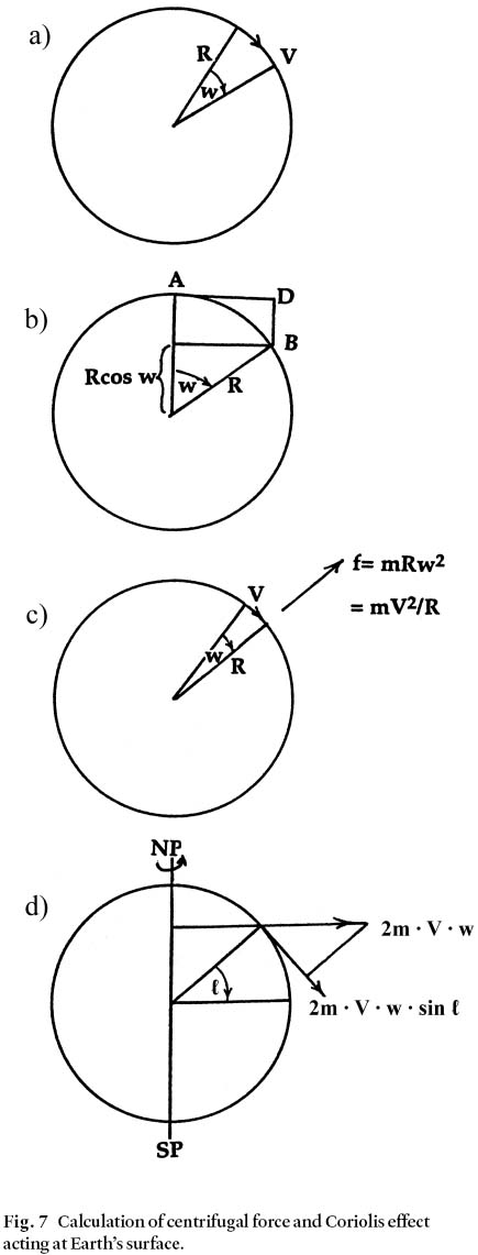
1.4.3. Applications to tides and water currents
51 Frictional coupling between moving water and Earth is weak except for a thin layer directly adjacent to the solid Earth. Consequently lateral water movements induced by tide generating forces respond readily to the Coriolis effect to an extent that is directly proportional to the mass and the speed of the object in question. Thus, one litre of water, having a mass of 1 kg, and moving at a speed of 1 ms -1 (1.944 knot) in relation to the Earth at 45°N latitude, will be moved to the right of its original direction. It will have been deflected by the Coriolis effect with an acceleration of:


Dimensions: W m, k = 1852 m/hr = 0.5144 ms -1 = 1 knot
52 In the Bay of Fundy and elsewhere, tidal ranges in wide stretches of water with strong tidal currents will be higher on the side of the channel that is to the right of the flood tide. When the tide reaches its peak level at any segment of the tidal estuary or channel, except for the uppermost reach of the tide, the water continues flowing landward because waters in the upper reaches will still not have reached their maximum level. Some time is required before the tidal current in the upper reaches comes to a standstill and then reverses. When the highest level is reached, the incoming tide will be higher at the right bank than at the left bank. Thereafter the water will be at a lower level and falling. In some instances the ebb current may be faster than the inward flow, causing a steeper lateral slope, but at a lower level. However the incoming tide will be more concentrated at the right bank. In the Bay of Fundy this will be at the southern or Nova Scotia side of the Bay, while the outgoing tide will be higher at the northern or New Brunswick side, resulting in an anticlockwise movement of the bulk of the tidal water.
53 Charts of the Bay of Fundy indicate that near Saint John, N.B., the Bay is 57 km wide. Tidal currents in that region have an average incoming velocity of 1.7 knots or 0.875 ms -1. Under these conditions the lateral water surface gradient due to the Coriolis effect can be calculated from equation (18) as:

54 At High Water in Saint John, the water continues to move towards the head of the Bay, where High Water occurs some time later. Assuming the current has a speed of 0.8 knots (0.4 ms), the outcome again can be calculated from (18) as:

55 Current speeds decrease after the water starts rising above Mean Water Level, and the movement correspondingly accelerates less. When acceleration to the right has ceased, the velocity to the right has to be counteracted by an opposite acceleration, either by the water moving in the opposite direction, or by the slope caused by the Coriolis effect. Eventually the water accumulated on the right side will start to move to the left. This movement causes a residual anticlockwise movement of the water in the Bay of Fundy and the Gulf of Maine as recorded by the movements of drift bottles. The phenomenon has been attributed to freshwater discharge of tributary rivers. However, compared with the tidal exchange, freshwater discharge is minuscule and of little account in the generation of residual currents.
56 The distance between Cape Cod and Cape Sable along the great circle is 414 km. The current speed in the Northeast Channel and over the Georges Bank may reach 2 knots or 1 ms -1. Theoretically, water levels at the Nova Scotia side could be more than 4 m higher ( H = 414000 · 2 sin 42.5° /130732 = 4.28 m) than at Cape Cod when the water surface is near mean water level. Near High Water the currents are not as strong and the Coriolis gradient correspondingly less. However it seems likely that the Coriolis effect contributes to much stronger tides along the Gulf of Maine coastline of Nova Scotia than near Cape Cod and the Great South Channel (between Nantucket Shoals and Georges Bank). The range of the tides on the Nova Scotia side varies between 2 m on the Atlantic Ocean side to 4.5 m near the entrance to the Bay of Fundy, while on the Cape Cod side it varies between 0.5 and 1.0 m. Even at the head of the Bay of Fundy there is a substantial Coriolis effect on water levels. For example, hydrographic charts show that in the 5300 m wide Minas Channel, currents of 8 knots can occur. This means that on one side of the Channel the water levels could be about 0.23 m higher (H = 53000 · 8 · sin 45°/130732 = 0.23m) than at the other side, because of Coriolis gradients.
57 The swing of the Coriolis effect with incoming tides might therefore be expected to exert a relatively stronger erosive power on southern or southeastern shores of channels and estuaries in the Bay of Fundy than ebb tides do on the opposite sides. In estuaries, of course, this swing is in the opposite sense to that of stream flow. Therefore, in Bay of Fundy estuaries at such times as stream discharge is relatively high, lateral mixing of fresh water and saline water will be promoted by the Coriolis effect.
58 The Coriolis effect is joined by the constraining effect of landmasses in imposing amphidromic systems on the tides (Fig. 8). Amphidromic systems occur in individual basins, seas, and lakes, for example the Gulf of St. Lawrence, or Lake Geneva on the border of Switzerland and France. In the elon-gated Lake Geneva, a gravitational forces cause a seiche, with alternately higher levels at one side than the other. In the Gulf of St. Lawrence, which is a more rounded body of water, the tidal movement is generated and kept going mainly by the ocean tides that enter through the Cabot Strait, with higher levels being at the right-hand side of the inflow. This results in the surface of the entire Gulf resembling a wobbling plate on a flat surface, with the highest (or lowest) rim of the plate rotating anticlockwise. In both cases the dimensions of the bodies of water must be such that a harmonic oscillation can take place. In the Gulf, the Coriolis effect causes a tidal wave to move anticlockwise, being high in the Cabot Strait when the ocean tide peaks. Dynamic tidal analysis thus treats tides as standing waves. The tides themselves are generally classified in terms of the ratio of the total amplitudes of the two principal diurnal components to the total amplitudes of the two principal semidiurnal components (for details see Fig. 4-3 in Desplanque and Mossman 1998a).
Fig. 8 In an amphidromic system developed in a bay in the northern hemisphere the flood tide (a) is deflected to the right, and the ebb tide (b) to the left by the Coriolis effect; (c) shows the result in cross-section. In (d) the tidal crest is shown at co-tidal lines for hour 3; motion of tidal crest is shown by arrow upon the water surface. "A" marks the (no tide) amphidromic point. Modified after OPEN (1993).

Display large image of Figure 8
59 When the declination of the Moon is at its maximum value of 28.96°, the Moon at its average distance from Earth will cause a maximum clockwise displacement of water particles around the poles of 438.5 m. If there were no Coriolis effect (i.e. if Earth were not rotating) the radius of the circular movement would be 146.1 m. The Coriolis effect thus tends to increase substantially the clockwise movements in the Northern Hemisphere, especially at points closer the North Pole. It has a much lesser effect on the anticlockwise movements that occur just north of the Equator. It is nil at the Equator, and maximum at the poles.
60 Note that although in the ocean basins anticlockwise motion of tide waves about amphidromic points occurs in the Northern Hemisphere, and vice versa in the Southern Hemisphere, several exceptions exist. The reason for these exceptions lies in the behaviour of the cotidal lines linking two amphidromic points. An example occurs in the southeastern Atlantic-western Indian Ocean system; here, as eloquently illustrated by Railsback (1991), amphidromic points linked by cotidal lines are likened to intermeshed gears (Fig. 9), and as such must necessarily rotate in opposite directions. This concept is particularly useful in explaining the anomalous sweep of the tides in low latitude systems.
Fig. 9 In this illustration of amphidromic systems as gears, all amphidromic points are linked by co-tidal lines. All independent systems (e.g. south of 30°S) rotate clockwise as predicted by the dynamical theory of tides and the Coriolis effect. After Railsback (1991), with permission.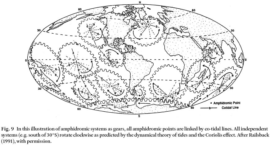
2. Regional Tides (TOP)
2.1. TERMS OF REFERENCE
61 Defant (1958) described tides, colourfully, as "… the heartbeat of the ocean, a pulse that can be felt all over the world." More technically, "tide" is the periodic rise and fall of the ocean surface in response to gravitational forces of the Moon and Sun. The periodicity of the tides is imposed by astronomical cycles determined by the relative motions of the Earth, Moon, and Sun. The regularity of tidal movements makes accurate prediction possible, and sets tides apart from other changes in sea level and from irregular phenomena like earthquakes, storms, and volcanic eruptions. In practice, tides are a mixture of diurnal (daily) variations, with one low and one high tide each day, and semidiurnal (twice daily) variation with two low and two high tides each day. In relatively shallow coastal waters these motions are of course greatly magnified. The "range" of the tides generally refers to the vertical movement of the water surface between the Low Water and the High Water levels of the tide. This factor, and the regime or mixture of the two types of tides varies from one area to another and also over time at any given location.
62 In Canada, the tidal levels in use (Canadian Tide and Current Tables 2004) are:
- MWL – Mean Water Level – average of all hourly water levels observed over the available period of record; in comparison, Mean Sea Level (MSL) is a statistically established entity.
- HHWLT – Higher High Water, large tide – average of the highest high waters, one from each of 19 years of predictions.
- HHWMT – Higher High Water, mean tide – average of all the higher high waters from 19 years of predictions.
- LLWMT – Low Low Water, mean tide – average of all the lower low waters from 19 years of predictions.
- LLWLT – Lower Low Water, large tide – average of lowest low waters, one from each of 19 years of predictions.
- LNT – Lowest Normal Tide – in present usage it is synonymous with LLWLT, but on older charts it may refer to a variety of low water chart datums – it is also called Chart Datum (CD), a most important term of reference.
63 All tidal measurements are made from the local Chart Datum (CD), an elevation so low that the tide at that place will seldom if ever fall below it. Thus, soundings on hydrographic charts show mariners the minimum depth of water. The tidal range gives them an extra margin of safety. Generally the tidal range is small and so is the margin of safety. However, for the Bay of Fundy, on charts showing a number of tidal stations, the difference between Chart Datum and Mean Water Level in one section of the charted area may be quite different than it is in other sections. The soundings on such charts do not allow one to construct a proper three-dimensional picture of the shape of the Bay. On land, the datum used by geodesists, surveyors, and engineers is the Geodetic Survey of Canada Datum (GSCD, or GD). This datum is based on the value of mean sea level prior to 1910 as determined from a period of observations at tide stations at Halifax and Yarmouth, N.S., and Pointe au-Père, Quebec, on the east coast, and Prince Rupert, Vancouver, and Victoria, British Columbia, on the west coast. In 1922 the datum was adjusted in the Canadian levelling network. Because in most areas of the Maritime Provinces the landmass is submerging relative to mean sea level, geodetic datum drops gradually below mean sea level. However, there is a dearth of data, and no one is certain exactly what the difference is between GSCD and MWL at different stations. This situation is troublesome for engineers and biologists who need to know the proper relation between the two datums at particular places.
2.2. OVERVIEW OF REGIONAL TIDES ALONG THE EASTERN CANADIAN SEABOARD
64 Between the Atlantic Ocean and the eastern seaboard of the North American continent lies the continental shelf. In large measure a result of planation during the ongoing Pleistocene– Holocene Ice Age, the continental shelf has depths of less than 250 m. Near Cape Breton Island, it extends more than 200 km from the coast, although near the southern tip of Nova Scotia it narrows to 130 km (Fader et al. 1977). Farther south, along the coast of the United States, the shelf varies between 25 and 200 km. Off the continental shelf the seabed drops to depths of 5000 m over a distance of about 200 km. This 200 km-wide margin is known as the continental slope. Along the outer edge of the shelf the average tide ranges between 80 and 100 cm. After crossing the continental shelf, the tidal range along the shore of Nova Scotia is increased to between 120 and 140 cm.
65 When the relative positions of the Earth, Moon, and Sun generate exceptionally large tides, the tidal range along the shoreline of Nova Scotia may reach as high as 200 cm. This increase is 40– 50% above average. Conversely, when the relative positions of the Earth, Moon, and Sun are such that tides are weakened, ranges drop by about 40% below the average. Variations in tidal strength of 60% to 140% are observed in the Gulf of Maine and the Bay of Fundy (Fairbridge 1966).
66 Between the Gulf of Maine and the Bay of Fundy, along the edge of the continental shelf off southwestern Nova Scotia and Cape Cod, Massachusetts, a series of shoals and banks acts as a sill obstructing tidal flow (see Fig. 3); in places the water is barely 4 m deep. Three channels cross this sill, of which the Northeast Channel is by far the largest between ocean and Gulf. Located between Georges Bank and Browns Bank, it is 230 m deep, 40 km wide, and 70 km long.
67 Tides on the ocean side of the Northeast Channel have an average range of 90 cm, but 320 km eastward at Bar Harbor, Maine, they have a mean range of 310 cm. High Water on this part of the coast is 3 hours later than along the edge of the continental shelf. The strength of tides in the southern bight of the Gulf of Maine, up to Race Point off Cape Cod, is rather uniform, varying between 210 and 310 cm for average tides; however between Bar Harbor and Jonesport 50 km to the east, their strength steadily increases toward the upper reaches of the Bay of Fundy. The average tidal range at the entrances to Minas Basin, Cumberland Basin, and Shepody Bay, each about 320 km from Bar Harbor, is 960 cm. However, in the Minas Basin the tides are 100 minutes later than at Bar Harbor. Tidal ranges are greatest in the estuaries of the Salmon and Shubenacadie rivers in the Minas Basin, 400 km from Bar Harbor. Depending upon astronomical conditions, this average range increases to 1360 cm. To the dismay of many inhabitants along this coast, even this enormous tidal range may be greatly extended by storm conditions.
2.3. GRAPHICAL SYNTHESIS OF REGIONAL TIDES
68 Figure 10 (see appendix) shows the tidal ranges along the eastern Canadian seaboard during mean and large tides. At most places the tide reaches a maximum level on an average interval of 12.4 hours. Usually one of the two daily High Waters is higher than the other and is called the Higher High Water. Similarly, a Lower High Water and a Lower Low Water occur during a day-long tidal cycle. The distance that the tide moves up or down from the Mean Water Level is called the amplitude of the tide, and the total vertical distance between High Water and Low Water is the tidal range. The range given in the Canadian tide tables for a given locality is specifically for the distance between Higher High Water and Lower Low Water. This gives a somewhat larger value than ranges listed in American tide tables, which are calculated from the mean of the semidiurnal tides.
69 The center line of the band representing the tidal ranges (Fig. 10) depicts the local Mean Water Level; the pair of lines closest to this center line delineates the range during average tidal fluctuations in the area, and the outer pair delineates the fluctuation during large tides. Large tides occur when the main tide-producing astronomical forces are at maximum strength and working more or less in unison. The rise in feet of the Higher High Water above Mean Water Level during large and mean tides, and the fall of the Lower Low Waters below that datum, are shown on the chart beside the inserts which indicate the tidal characteristics near the principal tidal stations in the region.
70 Along the eastern Canadian seaboard the tidal ranges are rather uniform at 4 to 5 feet (1.22– 1.52 m). The smallest tidal ranges in the charted area are recorded on the west coast of the Magdalen Islands and in the western Northumberland Strait, with mean ranges of 1.5 and 2.0 feet (0.45 m and 0.61 m). However in embayments such as the Bay of Fundy, the Bay of Chaleur, the channel leading to the St Lawrence River estuary, and the eastern and central parts of the Northumberland Strait, tidal ranges gradually increase at points more distant from ocean tides (White and Johns 1977).
71 Tidal characteristics near the principal, or reference, ports (e.g., Halifax, North Sydney) are included as marigrams in Fig. 10. The examples show the predicted tidal movements for March, 1966, a date chosen arbitrarily, the particular astronomical conditions for which are given with the sample set in the legend (inset at lower left of Fig. 10). The marigrams for this month are typical of any monthly period except that the sinusoidal diurnal and semidiurnal variations are offset according to astronomical conditions. In order to accentuate these characteristics, different vertical scales are employed. For this reason the local tidal amplitudes of Higher High and Lower Low Water during large and average tides are printed to the left of the inserts (see "Typical Tidal Variations over one Month"). Note that ranges are largest shortly after full moon and new moon during spring tides. When the Moon shows its quarter phases, the amplitudes are small and the tides are neap. The influence of the distance of the Moon from the Earth is such that when the Moon is in perigee (closest to Earth), spring tides are higher than when the Moon is in apogee (farthest from Earth). The diurnal inequality between high waters and low waters is nil when the Moon moves through the plane of Earth's equator, and as seen from Earth, reaches its peak when the Moon is in its most northerly or southerly position in the sky.
72 Local tidal characteristics along the eastern Canadian seaboard result from a combination of diurnal tides and semi-diurnal tides. The diurnal tide repeats itself every 24.8 hours, and the semidiurnal tide every 12.4 hours (see insert, lower left hand side of Fig. 10). At most locations the semidiurnal tide is dominant. An exception is in the southern Gulf of St. Lawrence where, under certain astronomical conditions, only one High Water and one Low Water occur daily; here semidiurnal tides may have less than half the range of the diurnal component. Diurnal tides dominate along the north coast of Prince Edward Island, the west coast of the Magdalen Islands, and in the western portion of the Northumberland Strait.
73 Tidal characteristics also depend on the phase relationship between the diurnal and semidiurnal components. This manifests itself prominently in the Gulf of St. Lawrence where the strengths of both components are similar. Here there is less variation than in the Fundy tides, and there is no annual progression of 1.5 months in the highest tides. Tides in the Gulf of St. Lawrence tended to be higher in 1969 and 1973 (Fig.11), years of relatively low tides in the Bay of Fundy (Canadian Hydrographic Service 1964, 1969a, 1969b, 1973, 1979, 1981).
Fig. 11 Predicted maximum (Highest High Water) and minimum (Lowest Low Water) monthly water levels for The Gulf of St. Lawrence ports of Portage Island, Shediac Bay, New Brunswick, and Rustico, Prince Edward Island, over an arbitrarily chosen 8 year interval. Note that the HHW and the LLW occurred near the winter and summer solstices.
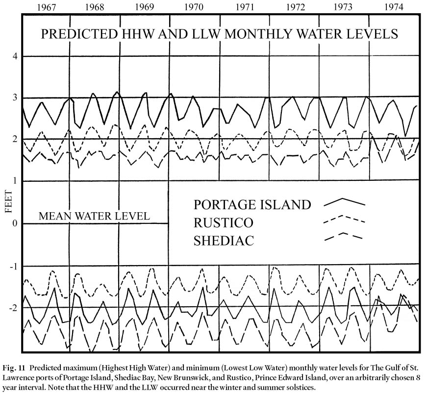
Display large image of Figure 11
74 Several other interesting contrasts exist among regional tides. In the Gulf of St Lawrence, when the High Water of a diurnal tide coincides with one of the two High Waters of the semidiurnal tide, the Higher High Water of the day is higher than the Lower High Water, assuming that the semidiurnal tide dominates at the location. This situation is because the other semidiurnal peak will coincide with the diurnal Low Water. Under these conditions the semidiurnal Low Waters will occur when the diurnal tide is near Mean Water Level and both will drop to almost the same level. This combination occurs in the western section of the Gulf of St. Lawrence (Fig. 10) where the High Waters at Rustico, P.E.I., Portage Island, N.B., and Pointe St. Pierre, Quebec, are usually unequal, in contrast to the almost equal Low Waters. (In Fig. 10 this is shown on the inserts indicating tidal characteristics near certain ports.) Note too, in Fig. 11, that the highest tides in the Gulf of St. Lawrence occur at mid-year and at year end, contradicting the age-old notion that equinoctial tides (March and September) will be the larger tides. Conditions similar to those of the Gulf of St. Lawrence prevail along the east coast of Newfoundland near St. John's and Argentia. The opposite conditions prevail in the Northumberland Strait where one of the semidiurnal Low Waters nearly coincides with the diurnal Low Water resulting in generally unequal Low Waters and almost equal High Waters (e.g., at Charlottetown, P.E.I., Pictou, N.S., and Shediac, N.B.). As shown in Fig. 12, for Halifax, North Sydney, and Charlottetown, the winter tides are predicted to be higher than summer tides. Note, too, that the Low Waters of Charlottetown extend much further below MSL than the High Waters reach above this level. This is because of the diurnal inequality of the tides, which causes High Water to be nearly the same each day and Low Water level to vary.
Fig. 12 Predicted maximum (HHW) and minimum (LLW) monthly water levels for the Atlantic Ocean ports of Halifax and North Sydney, N.S., and Charlottetown, Prince Edward Island, over an arbitrarily chosen 10 year interval. Note that in all years the HHW occur near the winter solstice, and the LLW near the summer solstice.
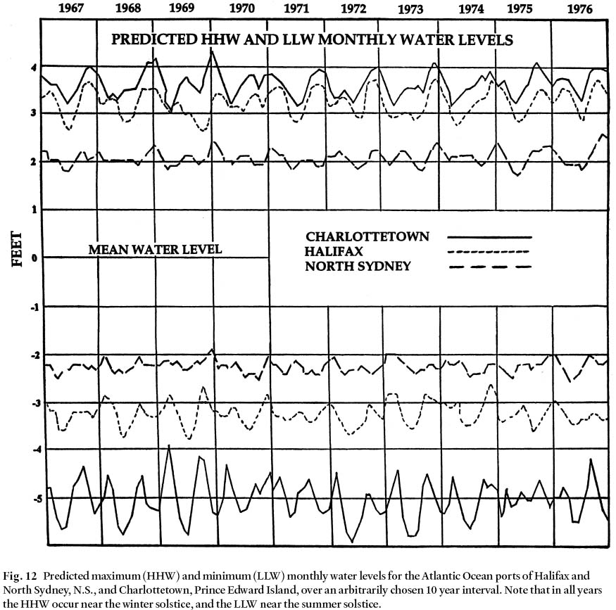
Display large image of Figure 12
75 As a result of the Coriolis effect, in large bodies of water such as the North Atlantic Ocean and the Gulf of St. Lawrence, the tides and especially the semidiurnal tides circulate along the surrounding coastlines in an anti-clockwise progression forming an amphidromic system. At and near the system's central point the tidal range is nil. The location of the amphidromic system in the Gulf of St. Lawrence is shown in Fig. 10. Farther removed from the central point the tidal range gradually increases. Illustrating this progression the chart shows (in lunar hours, 1 to 12) the approximate positions of High Water of the semidiurnal component of the tide in this system. This semidiurnal system splits at the western side of the Northumberland Strait, one wave going directly into the Strait and the other traveling around Prince Edward Island and moving partly into the eastern entrance of the Strait; as it moves westward to Shediac Bay (see Fig. 10), it meets the wave trough of the one entering the west entrance. The result is that the semidiurnal tide is scarcely noticeable in this area, and so the diurnal tide becomes dominant. Only when the Moon is near the Equator will semidiurnal tides be observed.
76 Tides in the Gulf of St. Lawrence are generated and maintained by tidal movements in the Atlantic Ocean. The two systems appear to be synchronized, with simultaneous High Waters and simultaneous Low Waters at their meeting place in the Cabot Strait. Thus, the diurnal tide in the Gulf maintains a see-saw relationship with that of the Atlantic Ocean, being high in the Gulf when it is low in the ocean. The Coriolis effect causes the diurnal tides to peak in the northeastern part of the Gulf before they reach their maximum level along the southwestern coastline.
2.4. ADDITIONAL CONSIDERATIONS
77 During spring and summer in the Bay of Fundy and in the Northumberland Strait, the Lower Low Water occurs during the daytime (and HLW at night!) so that the tidal flats absorb considerable heat from the Sun. As the tide rises over the warm tidal flats, the water temperature rises, especially in the Northumberland Strait where the water cover is comparatively thin.
78 During the same seasons, in the western section of the Gulf of St. Lawrence the Lower High Water occurs during the daytime, covering to a limited depth the Sun-heated beaches and shoals with almost the same temperature-raising effects as occur along the Northumberland Strait. This has ecological implications. For example, both sections of the Gulf have a mollusc fauna similar to that found near Virginia along the eastern U.S. seaboard. The species involved need a water temperature above 68°F (20°C) to spawn. Yet, even during the warmest months of the year the mean air temperature in the Gulf is less than this value. Tidal characteristics of the area are therefore probably important factors in the propagation of these species in this part of the Gulf.
79 Conditions are reversed during fall and winter, exposing tidal flats to heat loss at Lower Low Water during the night. This results in the following Lower High Water being cooled well below normal sea water temperature as it flows over these frigid flats, circumstances that probably aggravate ice conditions.
80 A tidal wave with a period of about 12.4 hours appears in the Atlantic Ocean in front of the Gulf of Maine, causing a wave to enter through the Northeast Channel. The wave propagates over the Gulf, reaching the shore about three hours later. As this progressive wave moves along the mouth of the Bay of Fundy, a standing wave is formed, and energy becomes concentrated toward the head of the Bay as its cross-sectional area is gradually reduced.
81 A standing wave can form in a basin in which the water moves periodically from one side to the other, high water at one side corresponding to low water on the other. The strength of the tide is strongest at the ends of the basin. Although in the center of the basin the water surface does not move up and down, strong currents are present because a large volume of water must move to and fro in order to create the High Water alternately at both ends.
82 The funnel-shaped Bay of Fundy branches at its northeast end into the Minas Basin and Chignecto Bay. The dimensions of the Bay of Fundy are such that its natural period of oscillation closely approximates that of the semidiurnal tidal component, thus greatly increasing resonance. There are fascinating variations on this theme. For example, as detailed in section 1.4.3 (on applications to tides and water currents), due to the Coriolis effect the entering tidal stream is deflected toward the southern shore of the Bay and the retreating stream to the north.
83 On average, the up and down sweep of the tide solely due to the Coriolis effect is larger on the Nova Scotia side for the incoming tide than for the outgoing tide on the corresponding opposite New Brunswick shore (see Fig. 13). Thus, when the water reaches its highest level (A), the tide is still coming in, filling the upper reaches of the Bay, and the water maintains a lateral slope AB (Fig. 13a). At the turn of the tide, it is level (BC), although the level on the Nova Scotia side will have already dropped (A to C). Note that, like the sweep of the tidal level due to the Coriolis effect, the range of the incoming tide in any Fundy cross-section is higher perpendicular to the axis of the Bay on the Nova Scotia side. Likewise, tidal flow entering the Gulf of Maine, results in a higher tidal range on the Nova Scotia side. The same argument applies to any cross-section as the tide ebbs (Fig. 13b). Approaching the turn of the tide, the water continues flowing seaward for some time, just as it still has kinetic energy which allows it to flow upward to higher level (D) on the New Brunswick side than on the Nova Scotia side (F). At the turn of the tide, it is level (DE).
84 Thus, the south shore experiences a greater tidal range than does the north shore, as well as a counter-clockwise system of residual tidal currents (see Fig. 13). Turbulent current in the narrow strait between Minas Channel and the Minas Basin can exceed 11 knots.
Fig. 13 Diagrams show, respectively for ebb and flow, the tidal levels across the Bay of Fundy from Nova Scotia to New Brunswick. The greatest slope in each instance occurs at mid-tide. Tidal range on the Nova Scotia shore is greater than on the New Brunswick shore in any cross-section perpendicular to the axis of the bay. Given is a 24.8 hour lunar day, with each semidiurnal tide being 6.2 hours long. See text for details.
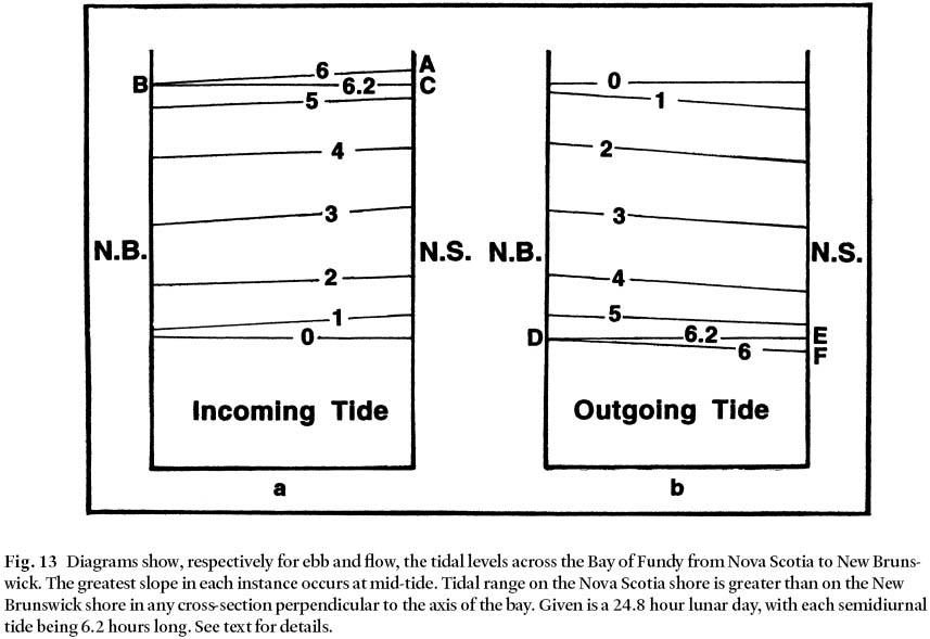
Display large image of Figure 13
85 In the upper reaches of the Bay of Fundy, the standing wave fills the estuaries. However, the rate of rise of tide is so rapid that large flows of water into the mouths of the estuaries would be required if the water surface in the estuaries were to rise at the same rate as in the Bay. Because the estuarine cross-sections are relatively small, particularly at low tide, such large flows of water are not able to enter. Therefore, filling of the estuaries is delayed. Physical restrictions on flow velocities are much more severe in shallow water than in deep water. The result is that water flowing in the more shallow parts is overtaken in time by water which, although entering the estuary later, moves faster in the deeper water. Thus, on the gently sloping bottom of the estuary a tidal bore commonly develops, most impressively so when the tide has its largest amplitude.
86 Theoretically, in basins where a standing wave occurs, hardly any currents are at the end where the tides are strongest. However, if there are shallow estuaries to be filled, strong tidal currents will develop in a relatively short time. These currents are the main agents of transportation and deposition of sedimentary materials in the Bay.
87 High Water occurs progressively later further up the estuaries. This High Water can happen quite a distance up the estuary, and considerably later than the time of High Water at the mouth. The time differential depends in turn on the gradient of the estuary bottom within the tidal range. As we shall see (section 9.5), these two factors are intimately linked to the evolution of the tidal marshes within estuaries in the Bay of Fundy.
2.5. A SUCCESSION OF STANDING AND PROGRESSIVE WAVES
88 A profound difference exists between the tidal regime of the Gulf of St. Lawrence and that of the Bay of Fundy. This much is evident in the frequencies and occurrence of monthly maximum and minimum tidal water levels. Predicted tide water levels over typical 8- and 10-year intervals are shown for three ports in, respectively, the Gulf of St. Lawrence (Fig. 11) and the Atlantic coast (Fig. 12). Note that in all years the highest High Waters for Charlottetown, Halifax, and North Sydney (i.e., the Atlantic coast) were predicted around the winter solstice (Fig.12), whereas the lowest Low Waters occurred near the summer solstice. However, for the three ports in the Gulf of St. Lawrence (Fig. 11), the highest High Waters and the lowest Low Waters occurred near the solstices, but with no noticeable difference between those near the winter solstice and those near the summer one. The smallest ranges of the tides were predicted to occur near the equinoxes.
89 The above relationships clearly demonstrate that the tidal regime along the Atlantic coast is different from that in the Gulf of St. Lawrence. Both are unlike the one in the Bay of Fundy. While in most waters, the largest tides occur in the same part of the year, in the Bay of Fundy they are more influenced by the shifting coincidence of spring and perigean tides with the result that each year they occur about 47 days later than in the previous year. Overall, regional tides along the eastern Canadian seaboard are best described as a succession of standing and progressive waves. The standing waves occur in the Atlantic Ocean, the Gulf of St. Lawrence, and the main body of the Bay of Fundy, whereas the progressive waves occur in the Gulf of Maine, the upper reaches of the Bay of Fundy, and in the estuaries leading into the Gulf and Bay. Progressive waves, unless supplied by external sources of energy such as air currents, do not grow in strength, for they lose energy when moving through confining channels. Likewise, progressive waves entering a restricted harbour mouth lose strength when they expand over the wider harbour surface. However, as we shall see, the wave entering the Gulf of Maine through the Northeast Channel seems to gain in strength while spreading over the Gulf. In fact it becomes 3.5 times stronger on reaching the shoreline.
3. Tides of the North Atlantic (TOP)
3.1. WATER PARTICLE MOVEMENTS
90 According to Pliny the Elder, writing in his Historia naturalis: "… tides swell more during the equinoxes, more during the autumn than in the spring, but… were empty at midwinter and even more so at midsummer". Unknown to Pliny, the tides are much complicated by the shape of the oceanic basins. The example of conditions prevailing in the North Atlantic on 5 September, 1975, with the new moon in perigee (and rather small declinations of the Sun, 6.5°, and Moon, 5.8°) serves very well to illustrate (Clancy 1969). With the Moon closest to Earth on its monthly orbit, higher than normal tides can be expected. The theoretical movements of individual particles in the ocean on this date (for details see Desplanque and Mossman 1998a) are rather small, clockwise, and predominantly diurnal. Nevertheless, the tides on that day were large. Table 4 provides the times and heights of the tides as they were predicted to be at sixteen ports along the eastern seaboard of the North American continent.
91 Do movements of the North Atlantic ocean follow water particle movements generated locally, or are they a result of an oscillating motion of the ocean with a period of 12.4 hours? First let us compare the times of High Water with the location of water particles in their cycle near 45° N latitude.
92 Table 4 shows that the highest tides on the western side of the Atlantic reach the highest levels of the day between 18:45 and 20:49 AST (moving from north to south, as indicated by the theoretical particle movements calculated for that day). The smaller high tides for that day occurred between 6:30 and 8:30 AST.
Table 4. Tides predicted for 5 September, 1975, along the eastern seaboard of North America
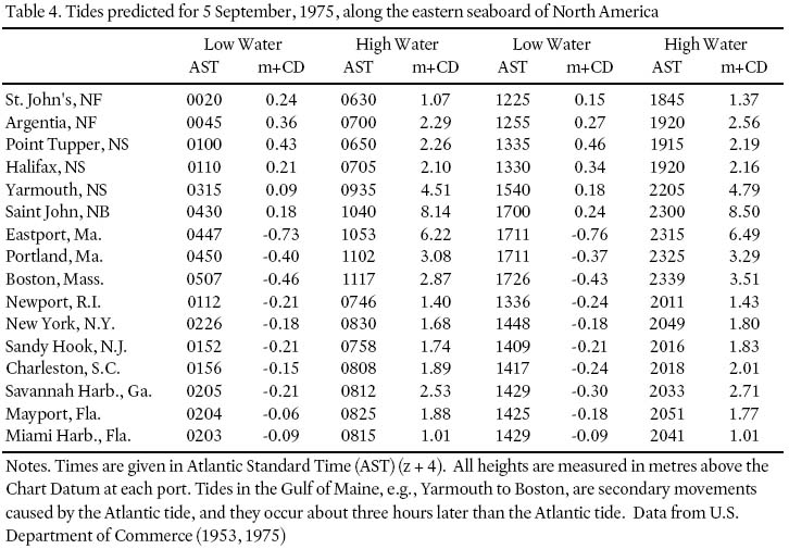
Display large image of Table 4
93 Semidiurnal tides are predominant in the Atlantic Ocean, the diurnal component being small (Fairbridge 1966). On the eastern side of the Atlantic (Table 5), the diurnal inequality of the tide is small. The High Waters from Morocco to France (about 15°N and 45°N latitude respectively) occur between 9:40 and 11:35 AST (13:40– 15:35 GMT) and 22:00 and 24:50 AST (2:00– 4:00 GMT), the tidal wave moving from south to north (Schwiderski 1980). These times coincide closely with those for the easternmost locations of water particles (Desplanque and Mossman 1998a).
Table 5. Tides predicted for 5 September, 1975, along the west coast of North Africa and Europe
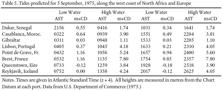
Display large image of Table 5
94 Given the Atlantic Ocean's 5000 km width and 5000 m depth, a scale model of this ocean as an oscillating basin would be approximately 1 m square and 1 mm deep. As it turns out, such a model is unrealistic (see Kwong et al. 1997) although it clearly illustrates the shallowness of the ocean. For example, if the ocean is oscillating, then when the water is high at one side of the ocean it should be low at the other side. So, if it is high between 9:40 and 11:40 AST (Table 5) at the eastern side one should expect it to be low at the same time on the western side. However, according to Table 4, low tide occurs in the west between 12:25 and 14:29. It appears, therefore, that ocean tides are more in tune with water particle movements than with an oscillating system.
3.2. TIDAL CONSTITUENTS AND HARMONIC ANALYSIS
95 Except for the Gulf of Maine and the Bay of Fundy, the ranges of tides on the eastern side of the Atlantic Ocean are substantially greater than those along the North American coast (Apel 1987). Harmonic analysis, the principle first applied to tidal problems by Lord Kelvin (1824– 1907), is the most satisfactory method of comparing characteristics of tides observed at various locations (Schureman 1941, 1949; Fairbridge 1966). This method relies on the fact that the observed tide is the result of several astronomically driven partial tides. Just as complicated sea waves can be reconstructed by combining several wave trains, so also can tides be calculated by combining partial tides, or tidal constituents. For most ports bordering the North Atlantic Ocean (Desplanque and Mossman 1998a), the M2 constituent is dominant (see Table 3; Fig. 14).
Fig. 14 Location of selected tidal stations in the North Atlantic ocean along the east coast of North America and along the west coast of Europe and North Africa, and of temporary gauging stations across the Atlantic.
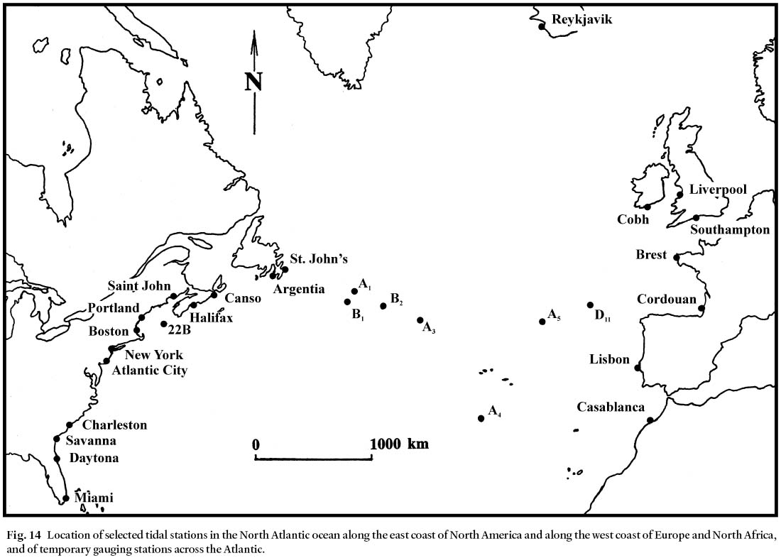
Display large image of Figure 14
96 Since 1977, tidal records have been collected along the edge of the continental shelf off North America, and more recently at several stations in the mid-Atlantic between Newfoundland and Portugal. Tables 6 and 7 show the results of analyses of these data together with data from shore stations. The ranges of the major constituents at these stations are given and the strength of other constituents is compared with M2. This can be used to determine if the local S2 tide is close to its theoretical strength of 46% of the M2 strength.
97 The value of the initial phase p (known as the phase lag and representing the phase of the constituent at the time of origin) is given as the epoch (Table 6), based on the local meridian of the observation station, and the 65°30' W meridian. The use of the latter as a time meridian is prompted by the fact that this meridian crosses the main entrance of the Gulf of Maine and also the entrance of the Bay of Fundy. Note in Table 6 that the percentage of S2/M2 is close to the theoretical value of 46% near Newfoundland, but slightly less in the eastern North Atlantic. The relative strength of the N2 constituents remains close to 22%, while the already weak diurnal K1 and O1 constituents are even weaker in mid-ocean. One might expect that the tidal wave would follow the apparent westerly movements of agents that account for the existence of the various constituents. However the phase lags indicate that the co-tidal lines move from west to east, in the opposite direction of the imaginary heavenly bodies.
Table 6. Characteristics of the tides, measured at mid-Atlantic stations between St. John's Newfoundland, and Lisbon.
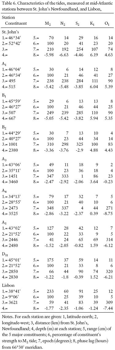
Display large image of Table 6
98 Table 7 shows the same type of data for ports along the eastern seaboard of North America, with additional data from some stations offshore. Indications are that the time of High Water is virtually the same for all stations over a distance of 2200 km between Banquereau Bank, south of the Cabot Strait, and Charleston, South Carolina. The strength of the Sun's influence is much less than the theoretical 46% of the Moon's influence, dropping from 24% at the Banquereau Bank to 17% at Charleston. Again there is little change in the relative strength of the N2 constituent. Thus, variations in the tidal strength caused by the variable distance between Earth and Moon gain in significance over variations in the influence of the Sun's gravitation. Stated otherwise, the perigean tides become more important than the spring tides.
Table7. Characteristics of the tides as measured along the edge of the continental shelf and at some ports along the east coast of North America
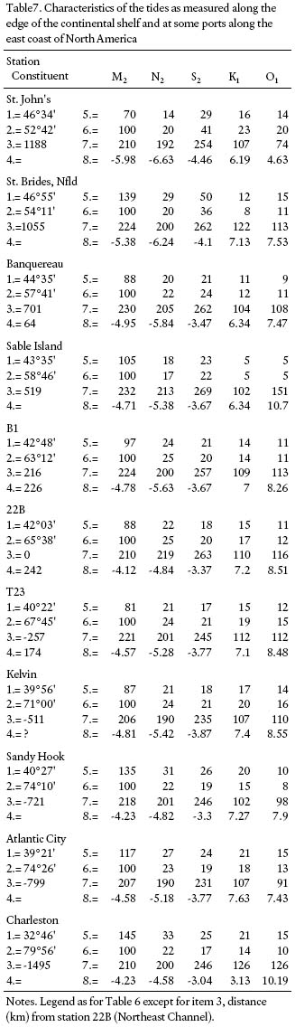
Display large image of Table 7
99 The influence of the Sun is far more noticeable along the coast of Newfoundland and Labrador. The percentage of S2 with respect to M2 ranges from 36% on the south coast of the Avalon Peninsula, north of the Cabot Strait, to 68% near Fogo Island at the northeast corner of Newfoundland. It drops again to 50% near the northern tip of the island, and to 36% along the Labrador coast. Evidently tides near Newfoundland have characteristics in common with those in the mid and eastern North Atlantic whereas tides south of the Cabot Strait have a different pattern.
3.3. EQUINOCTIAL TIDES: EAST VERSUS WEST
100 Other characteristics also indicate that tides between Newfoundland and Europe are of a different regime than those along the North American mainland. One of these characteristics concerns the stronger equinoctial tides. Plinys oft quoted statement probably accounts for the assumption by most oceanographers that the so-called equinoctial tides (March and September) reach higher levels than tides close to the solstices (June and December). Pliny may have been correct, for he was only aware of tides that can be observed on the east side of the Atlantic Ocean. Table 8 shows the highest predicted tides for each month in 1953 and 1975 for stations on the east side of the Atlantic. The semi-annual peaks are underlined. These data support Pliny's claim that the tides near the equinoxes are generally higher than those occurring during the remainder of the year. Even the fall tides are stronger than those in the spring, and the midwinter ones are stronger than the midsummer ones. However, as shown below, Pliny's claim is not valid along the east coast of North America, or along the continent's west coast south of the Alaskan panhandle.
Table 8. Highest High Water predicted for each month for ports on the eastern side of the North Atlantic Ocean

Display large image of Table 8
101 Data for 1953 and 1975 from stations on the west side of the Atlantic (Table 9) are rather less supportive of Pliny's case. However, in order to test for possible bias in the two sample years, Table 10 supplies a more complete set of data for Halifax. Note that the peak tides do not fall in the same months as they did on the other side of the ocean, and that they are spread over all seasons. The only month in which no peak occurs is September, one of the equinox months. Each successive year the peak appears to arrive somewhat later. This can be explained by the dominance of perigean tides on the west side of the ocean. The Spring Tide cycle has a period of 14.77 days, and the perigean cycle one of 27.56 days. After 205.89 days, these cycles overlap each other causing interference and extraordinary strong tides. Every second overlap occurs the following year, but 47 days later in the season. It is, therefore, incorrect to claim that on the western side of the ocean the equinoctial tides are the highest tides of the year. The highest tides of the year occur in the late fall and early winter season, because the mean water levels are higher in winter than in summer due to world-wide shifts in atmospheric pressures. Another phenomenon discernible in Table 10 (last column) is that every 4 to 5 years the tides reach another peak. This peak occurs because after 112 cycles of Moon declinations, their peaks occur again at almost the same time. The result is a 4.53 year cycle of extraordinary high tides.
Table 9. Highest High Water predicted for each month for ports on the western side of the North Atlantic Ocean

Display large image of Table 9
Table 10. Highest High Water predicted for each month for the port of Halifax, Nova Scotia
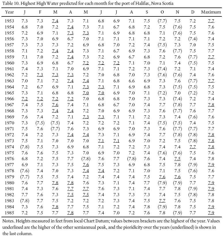
Display large image of Table 10
102 As discussed earlier, the theoretical movements of water particles in the oceans, due to the direct gravitational effects of the Moon and Sun, generally result in diurnal loops. Only during either new or full moon close to the equinoxes do strictly semidiurnal movements occur near the Equator. During fall and winter the most westerly displacements are reached during the morning hours, and during spring and summer in the evening hours. The diurnal inequality of tides along the North American seaboard shows the same tendency. During the summer months the most easterly displacements are reached around 04:00 and 05:00 hours local time, and during the winter, around 16:00 and 17:00 hours. As shown in Table 11 the tidal observations along the eastern side of the ocean are not in step with these particle movements. Clearly, tidal characteristics on the eastern side of the Atlantic differ significantly from those on the western side. It seems likely that the North American ocean basin, with its Sohm, Hatteras, and Nares abyssal plains, enjoys its own tidal regime, distant from that of the basins between Newfoundland and Europe.
Table 11. Diurnal inequality during solstices in 1953 on both sides of the North Atlantic Ocean
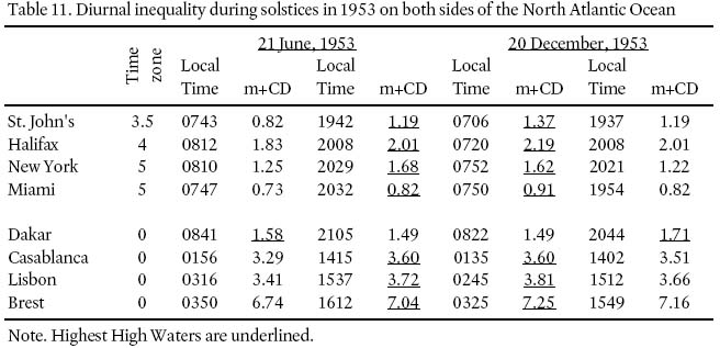
Display large image of Table 11
103 We turn now to the behaviour of tidal waters along the coast of northern New England where North Atlantic tides impinge on the Gulf of Maine and the Bay of Fundy.
4. Tides of the Gulf of Maine (TOP)
4.1. A DEGENERATE AMPHIDROMIC SYSTEM
104 Like the rest of the continental shelf, the Gulf of Maine results from drowning of the coastline due to the postglacial rise in sea level. The tides which beset its shores are perhaps best described as a degenerate amphidromic system. The amphidromic point, if such existed, would lie southwest of Cape Cod. However, the waters are too deep in the Gulf, considering its area, for a full amphidromic system to develop. Thus the tides of the Gulf of Maine are generated by the tides of the North Atlantic Ocean rather than directly by the Sun and the Moon. According to Redfield (1980) "The coast of New England north of Cape Cod opens on the Gulf of Maine where the behavior of the tide determines the tide in the numerous passages along the coast." In effect, the Gulf of Maine and the Bay of Fundy should be viewed as a single tidal system.
105 As mentioned previously, fronting the Gulf of Maine, at the edge of the continental shelf, is a natural sill which separates ocean from Gulf. This sill consists of a sequence of shoals and banks running from Cape Sable at the southern tip of Nova Scotia to Chatham on Cape Cod. Water that fills the Gulf of Maine between Low Water and High Water must move over the sill or pass through three channels between the banks (Apollonio 1979). Figure 15 shows the location and length of the sill along a line that approximately follows its shallowest parts.
4.2. SILLS, BANKS, AND CHANNELS
106 The distance along the shallowest part of the sill fronting the Gulf of Maine is 589 km, although the great circle distance between Cape Sable and Cape Cod is only 414 km. The crest of the sill runs from Nova Scotia, over German and Browns Banks, continuing on the other side of the Northeast Channel over Georges Bank, the Georges, Cultivator and Little Georges Shoals, and the Nantucket Shoals to Nantucket Island and Monomoy Island near Cape Cod. In places such as Georges Shoals there is barely 4 m of water. Over much of its extent, Georges Bank, which forms the main part of the sill, is less than 60 m deep (see Fig. 15 and Table 12 for location of various features and place names).
107 Three channels through the sill provide the main connections between the Atlantic Ocean and the Gulf. They are:
- The Northeast Channel between Georges Bank and Browns Bank, which is over 230 m deep, 40 km wide and 70 km long.
- A channel 120 m deep and 15 km wide between Browns Bank and German Bank off Cape Sable.
- The Great South Channel between Georges Bank and Nantucket Shoals.

Display large image of Figure 15
Table 12. Locations along a cross-section of the sill separating the Gulf of Maine from the North Atlantic ocean
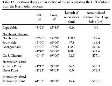
Display large image of Table 12
108 The shallowest parts of Browns Bank are small in area. The largest opening in the sill is between Georges Bank and German Bank; thus most of the water moving in and out of the Gulf of Maine flows through the section formed by the first two channels. Using bathymetric and hydrographic charts of the area, the width of the passage and its cross-sectional area at and below certain levels can be estimated. Because the Northeast Channel is the main passageway, these data are provided for the entire sill and for the Northeast Channel only (Table 13).
Table 13. Width and cross-sectional area of the water passage through the Northeast Channel, and over the sill separating the Gulf of Maine from the Atlantic Ocean
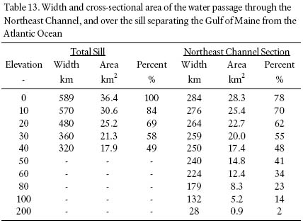
Display large image of Table 13
109 Approximately 80% of the available cross-sectional area is in the Northeast Channel section. Flow through this section has less friction to overcome than over the shoals, marked as they are in heavy weather by strong tidal currents and dangerously high seas. Thus an estimated flow of 80% through the Northeast Channel section is almost certainly a minimum.
110 The Gulf of Maine has a surface area of approximately 95 000 km 2, not including the 13 000 km 2 of the Bay of Fundy (Conkling 1995). Average depth of the Gulf is about 150 m. Within the Gulf are 21 basins, of which Georges Basin (maximum depth 377 m), Jordan Basin (304 m), Crowell Basin (304 m), and Wilkinson Basin (280 m) are the most prominent. These basins are separated by ridges and swells where the depth is between 150 m and 200 m. Along the 1100 km shoreline is a shallow fringe with depths less than 80 m. In detail, the shoreline is replete with numerous bays, islands, and tidal estuaries, its total length approaching 8000 km (Pilkey et al. 1989).
4.3. TIDES PRE- AND POST-PLEISTOCENE
111 In the millions of years before present that the Gulf of Maine was above sea level, subaerial erosion reshaped the exposed lowlands. Much of the sediment deposited during the early Cenozoic was removed, and valleys and deep stream beds were carved. The steep northern slope of Georges Bank may have been formed at this time. The main drainage outlet of the area was probably directed through what is now the Northeast Channel region.
112 Throughout the Pleistocene epoch, glaciers advanced and retreated several times on a global scale, deepening and widening valleys as well as causing sea-level fluctuations. Sea level dropped about 120 m as the last glacial advance removed water from the oceans, transferring it to continental glaciers. Advancing ice sheets were deflected eastward at the scarp-like northern edge of Georges Bank, and flowed as huge valley glaciers through what is now the Northeast Channel (Grant 1989; Keen and Piper 1990). On retreat, the ice left extensive terminal moraines and large areas covered with glacial out-wash. These and numerous other trademark glacial features have survived the drowning of this coastline by the postglacial rise in sea level.
113 Clearly, when the Gulf of Maine area was dry land, or covered with ice, the local tide action was of totally different character than it is now. At present, the amount of water exchanged during a tide of average strength within a 12.4 hour cycle, between the Atlantic and the Gulf, is about 300 km 3. Of this total, about 100 km 3 moves in and out of the Bay of Fundy. During the largest possible tides these amounts can be as much as 1.4 times average.
114 The watersheds of rivers flowing into the Gulf of Maine and the Bay of Fundy discharge about 95 km 3 per year, or 0.135 km 3 per tidal cycle. This is approximately 0.045% of the tidal prism of an average tide. Even during the spring when the river discharges can be ten times average, it is doubtful whether such a relatively small river flow can influence the circulation pattern in the Gulf.
115 During an average tidal cycle lasting 6.2 hours (22 357 seconds), flow through the available cross-sectional area of 36 km 2 needs on average to be only 0.37 ms -1 (0.73 knots) to fill the Gulf with ocean water. Assuming a harmonic motion, represented by a sine curve, the maximum current speed is 0.59 ms -1 (1.14 knots). This speed can be generated if a mass is dropped 1.8 cm at the surface of the Earth. It can also be caused by a column of water 1.8 cm high. Thus, if the water in the ocean is 1.8 cm higher than in the Gulf, the maximum velocity into the Gulf can be generated. At the seashore the average amplitude of the tide is 0.45 m. At mean sea level where the current is fastest, such a tide can rise 1.8 cm in 280 seconds (i.e., less than 5 minutes) (DeWolfe 1981). Therefore in order to receive all the water required to follow the ocean tide, the water surface in the Gulf has to follow the surface of the ocean by only 1.8 cm difference and less than 5 minutes in phase.
116 It has been argued that as the last glacial waned there was a time during which sea level was too low to allow tides of the present dimensions. The argument is that Georges Bank and other shallows were dry at the time, shortening the length of the opening. However, the remaining cross-sectional area in the Northeast Channel was still large enough to convey the water required to generate tides comparable to those today. The time lag would have been about 4 to 5 times larger than it is now but still small enough to prevent an appreciable change in the tidal regime.
117 Water entering the Gulf of Maine through the Northeast Channel moves as a wave through the channel, spreading quickly thereafter as a refracted wave throughout the Gulf. This wave travels 335 km to the coastline of Maine between Bar Harbor and Jonesport about 3 hours after entering the channel. Within half an hour, High Water will occur from Cape Cod Bay to the upper reaches of the Bay of Fundy except for Minas Basin, where there is a further delay of one hour.
118 According to Greenberg (1979) the average tidal range increases from 0.90 m at the entrance to the Northeast Channel to 3.10 m at Bar Harbor (Fig. 16). The ranges in the southern bight of the Gulf vary between 2.06 and 3.10 m, with High Water occurring a bit later. Stations in the center of the Gulf show intermediate ranges and times of occurrence. It seems remarkable that tides in the Great South Channel off Nantucket range from 0.63 m to 0.50 m, smaller than either ocean or Gulf.
Fig. 16 Locations of selected tide gauge stations along and near the coast of the Gulf of Maine and the Bay of Fundy. Average range of tides is indicated (in metres) for various stations and the time (distance) to High Water in hours in relation to the transit of the Moon through 66°30' W meridian (example 0.86/+0.26). WHOI = Woods Hold oceanographic Institute; UNH = University of New Hampshire. Modified from a computer simulation by Greenberg (1979) of the behaviour of the M 2 constituent.
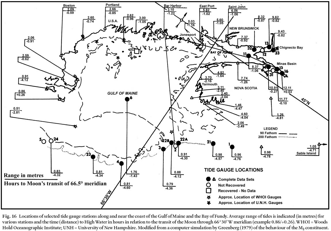
Display large image of Figure 16
119 Somewhere between Bar Harbor and Jonesport the tides assume a different character. Instead of having almost identical ranges as in the southern bight, the tidal range increases steadily in an east-northeasterly direction, reaching a maximum in the Minas Basin, 320 km from Bar Harbor. Here the highest High Water levels are reached in the estuaries of the Salmon and Shubenacadie rivers near Truro, about 400 km from Bar Harbor.
120 Between Cape Sable and Tiverton at the end of Digby Neck, the average tidal range increases from 2.13 to 4.80 m over a distance of only 115 km. Tides in this stretch of the Gulf shoreline of Nova Scotia adjust to the fact that the main thrust of the tidal wave is directed toward the Maine coast near Bar Harbor. The Gulf shore of Nova Scotia provides a short cut for the Fundy tides, resulting in a greater than usual increase in range per unit of distance along the shoreline.
121 A computer simulation developed by Greenberg (1979, 1987) of the behaviour of the M2 constituent indicates that the amplitude of M2 over Georges Bank and the Nantucket Shoals is the least of all (Fig.16), decreasing to as little as 0.25 (0.51/– 2). The close co-tidal lines between Georges Bank and Nova Scotia indicate the progressive wave character of the tide in that area, while the long distance in the southern bight and the Bay of Fundy indicates more of a prevailing standing wave (Greenberg 1987). High Water occurs last over the Nantucket Shoals and in the upper reaches of the Minas Basin (see Fig. 17). Standing waves in bays like Fundy, open-ended to the Gulf of Maine, behave much differently than standing waves in closed basins. From the edge of the continental shelf to the Minas Basin the tide takes from 3.3 to about 4 hours, an interval approaching a quarter of the oscillation period of the combined Gulf and Bay, accounting for the large tidal amplitude of the region.
Fig. 17 Computer generated tidal regime of the Gulf of Maine – Bay of Fundy – Georges Bank system. Behaviour of the M2 constituent reflects the change in character from a progressive wave at the entrance to the Gulf to a standing wave in the Bay of Fundy. Solid lines indicate the tidal phase in degrees, i.e., the progress of the tide as it arrives at the edge of the continental shelf. Broken lines show the tidal amplitude in centimetres, i.e., the predicted height of the tide above MSL. Modified after Greenberg (1979, 1987).
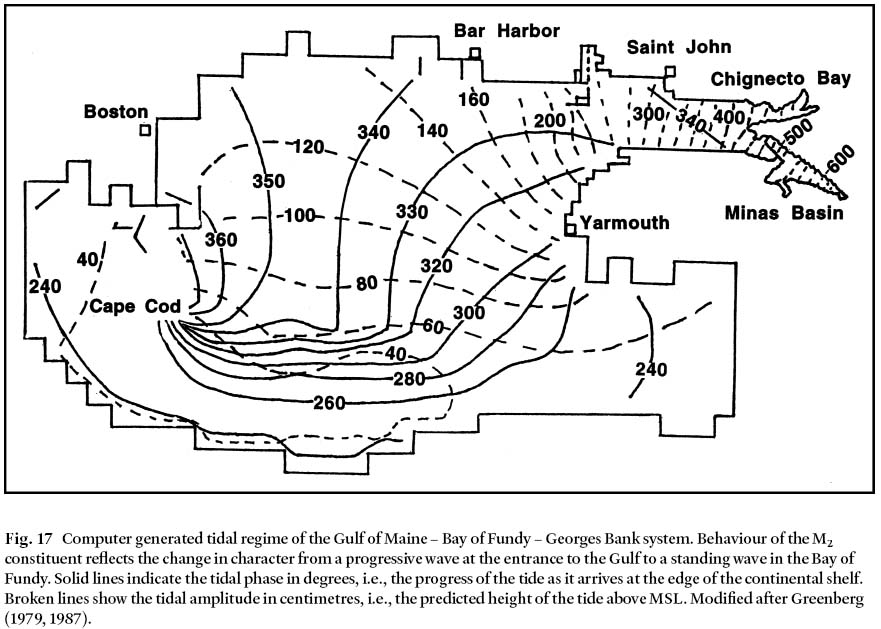
Display large image of Figure 17
122 The above considerations are of great importance in studies of tidal power generation because, among other things, construction of a tidal power dam in the Bay would lead to elevated tide levels. Controversy continues about the true resonant period of the Bay of Fundy, one problem in modelling being the determination of appropriate boundaries between Bay, Gulf, and ocean. Any major obstruction to tides in the Bay of Fundy would result in a change in the resonant period, which in turn could cause significant increase in the already extreme tidal amplification.
123 So much for the tides of a so-called "degenerate amphidromic system". Next we investigate the extent to which the Gulf of Maine and the Bay of Fundy act together as one tidal system resonating with the semidiurnal tides.
5. Tides of the Bay of Fundy (TOP)
5.1. INTRODUCTION
124 Bay of Fundy Tidal predictions are published annually for the principal hydrographic station at the reference port of Saint John. A mathematical approach using harmonic analysis is employed to compute the actual tide as the combined effect of all the tide-generating variables. The result is a large number of cosine curves, so-called tidal constituents or "partial tides", each representing the influence or characteristic of the local tide. Local tidal characteristics along the eastern Canadian seaboard result from a combination of diurnal and semidiurnal tides. However, semidiurnal tides are prevalent in the North Atlantic, and Fundy tides amplified by resonance across Georges Bank and through the Gulf of Maine are an integral part of the system (Gehrels et al. 1995; Davis and Browne 1996).
125 Recent observations of environmental characteristics of the Bay of Fundy suggest modern change in the dynamics of the system. They include the changing grain size distributions on the tidal mud flats (Amos et al. 1991), anecdotal observations from the fishing community of increasing water depths in some areas, and changing benthic communities (Percy et al. 1996). There is a need to better understand the dynamics of the Bay of Fundy and to promote efforts by concerned groups for a more detailed knowledge of seabed, oceanographic and biological conditions. Could the changes observed apply to the entire tidal regime? Are the tides stable or are they increasing due to changes in water depth or resonance length of the Bay? What is the future of the tides and associated currents in the Bay? These questions are central to the evolution of the Bay of Fundy and the sustainable management of its resources. In the following overview of the geology and evolution of the tidal regime in the Bay of Fundy, we elaborate on the tides at Herring Cove in Fundy National Park, N.B., and then examine the geological significance of the tides.
5.2. GEOLOGIC ORIGIN OF THE BAY OF FUNDY AND ITS TIDES
126 In strict terms, the Bay of Fundy is underlain by a half-graben with key faults on the northwestern margin. These faults, of Paleozoic or older origin, were reactivated at the onset of the opening of the present day Atlantic Ocean due to plate tectonic movements in the early Mesozoic (Keppie 1982; Greenough 1995; Withjack et al. 1995; Wade et al. 1996). Sedimentary infilling of the half-graben, termed the Fundy Basin, commenced with continental sedimentation about 230 Ma, during the Mid Triassic (King and MacLean 1976; Stevens 1977; Olsen et al. 1989; Withjack et al. 1998). During a late rifting stage immediately following the Triassic-Jurassic transition, voluminous basaltic lava erupted upon Triassic strata and was followed by mainly clastic sediment deposition possibly into the earliest Mid Jurassic (Olsen et al. 1989; Wade et al. 1996; Mossman and Grantham 1996). The entire sequence was then folded, uplifted and tilted southwestward in a saucer-shaped structure (Withjack et al. 1995). Thus rock exposures along the Fundy graben mark the boundaries of a major synclinal structure, the axis of which is located toward the center of the Bay. Mesozoic strata underlie much of the Gulf of Maine and the Bay of Fundy. Cretaceous sedimentary deposits preserved in isolated pockets in lowlands adjacent to the Bay of Fundy rest unconformably, usually on Carboniferous rocks (Stea and Pullan 2001; Falcon-Lang et al. 2003), suggesting that the Bay of Fundy Basin may have been covered by Cretaceous (and possibly Tertiary) deposits and subsequently exhumed.
127 In addition to basalt, much of the 1400 km coastline of the Bay of Fundy consists of erosion-prone sandstone and conglomerate. Erosion rates can exceed 1m/yr (Amos 1978), giving rise to sandy estuaries in which fine-grained clastic material accumulates in sheltered embayments. Some coastal sections of mainly Paleozoic siltstone and shale, for example in Chignecto Bay (Amos et al. 1991; Amos 1995a), contribute materials that persist in suspension through wave action and tidal cycling. Elsewhere, sections such as the basalt along much of the Nova Scotia coast, and the more massive igneous and metamorphic rocks along the New Brunswick coast, are relatively erosion resistant.
128 Glaciation has exercised important controls on the geo-morphology of the Bay of Fundy, as on its tidal regime. About 18 000 to 20 000 years BP, the Laurentide ice sheet blanketed most of Canada and extended far south of the Great Lakes. Crossing the Bay of Fundy and the Gulf of Maine, its approach to the edge of the continental shelf left blankets of glacial out-wash and huge terminal moraines peripheral to the ice sheet, as well as extensive drumlin fields. These deposits now form many of the banks and shoals along the Maritime and New England coastlines. Associated valley glaciers, such as one believed to have occupied the Northeast Channel in the Gulf of Maine, were also significant (Grant 1985, 1989; Keen and Piper 1990). During the last glacial maximum they contributed to a global sea level lower by 100– 130 m than at present. Overall then, there are two major phases to sea-level history in the Bay of Fundy: an early glacial emergence, and a present continuing submergence.
129 During the last 14 000 years the depth of the Bay of Fundy has changed appreciably as the land surface rebounded and sea level rose as the last ice sheets receded. One of the main features of the postglacial evolution of the Bay was the depth of water over Georges Bank; inflow of tidal waters was evidently restricted at the lowest point of relative sea level (Scott and Greenberg 1983). With progressive submergence of Georges Bank, the Bay of Fundy became more directly subjected to tidal forces. Mathematical modelling of the Gulf of Maine tidal system indicates that 7000 years BP, tidal ranges will have been 20– 50% of the present range (Greenberg 1979; 1987); by 4000 years BP they would have grown to 80%, reaching present strength about 2500 years BP, when mean sea level was approximately 7 m lower than present. There is general agreement too, that increasing erosion of the sea bed, with localized bottom scour and deepening, signals an increase in the dynamic energy of the tides (Bleakney 1986; Godin 1992; Fader 1996). However, the timing of increased resonance is controversial, because evidence from detailed salt marsh records indicates that tidal range was relatively subdued about 4000 yr BP (Shaw and Ceman 1999), a point earlier inferred by Grant (1970).
5.3. CHARACTERISTICS OF BAY OF FUNDY TIDES
5.3.1. Resonance and Range of Modern Fundy Tides
130 Impelled by the oceanic tide through the Northeast Channel and across the Gulf of Maine (Fig. 10), an average single tidal flow into the Bay of Fundy matches the estimated total daily volume (about 104 km 3) of all the world's river discharges into the oceans. Thus, during a lunar day (24 hours and 50 minutes), the water moving in and out of the Bay of Fundy is actually four times the combined discharge of all the world's rivers. During exceptionally high tides this volume may exceed 146 km 3 every 6.2 hours.
131 In effect, the tidal energy channelled into the Bay creates a slow, large-scale oscillation, or seiche. Tremendous tidal amplification may occur through this near-resonant response. A comparison with the pendulum movement of a grandfather clock is instructive. In this instrument, the visible movements of a heavy pendulum are maintained by an imperceptible downward-moving weight, keeping the pendulum going through the escapement mechanism. By analogy, the oceanic tides maintain a co-oscillating seiche, and thus the tidal movements in the Fundy - Georges Bank - Gulf of Maine system.
132 The appropriate formula describing these conditions (for an open basin like the Bay of Fundy) is given by:

133 Resonance in the Bay results in high tidal amplitude and a tidal range several times greater than the open ocean tide. Tides at Bar Harbor, with a mean range of 3.1 m, result from the increase in the mean range in the oceanic tides of 0.9 m, through the Northeast Channel and across the Gulf of Maine over a distance of 335 km. At the mouth of the Bay of Fundy (Fig. 3) the average range of the tides is close to 5 m, halfway into the Bay 7.3 m and at the head of Chignecto Bay near Belliveau Village, N.B., the average range is 12 m and can reach 15.2 m.
134 At Burntcoat Head, N.S., in Minas Basin near the head of the Bay (Fig. 3), the maximum range between successive low and high tides of 53.43 feet (16.29 m) was observed on 16 July, 1916 by Dr. William Bell Dawson, Superintendent of Tidal Surveys: this remains a world record. Here the mean range of 12.1 m is amplified about 13.5 times in relation to the oceanic tides over a distance of 735 km (Dawson 1920). The difference between high and low tide in the upper reaches of the Bay of Fundy is shown in Fig. 18.
Fig. 18 Views six hours apart, of tidal conditions in the Shepody River estuary, summer 1954, two years before construction of Shepody River dam near Riverside, N.B. Photographs by Con Desplanque.
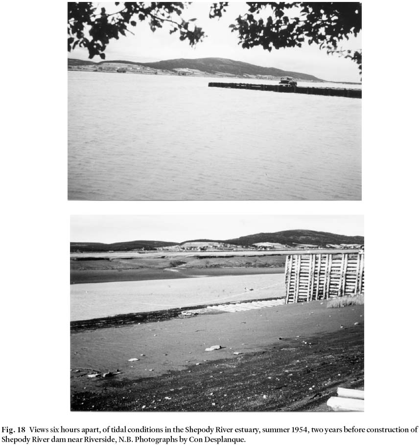
Display large image of Figure 18
135 Just northeast of the Jordan Basin is a threshold or sill of rock, which at its deepest point is 160 m below the present Chart Datum. This sill runs southeast from Jonesport, Maine, over the Grand Manan Banks, to a submerged continuation of Digby Neck (Lurcher Shoal), 40 km southwest of Briar Island (Fig. 19). In the 55 km wide channel between Grand Manan Island and Brier Island the water depth in places exceeds 200 m. Seventy-five kilometres farther into the Bay, on the line connecting Saint John, N.B. with Digby Gut, N.S., the depth is less than 100 m, while off Cape Chignecto, another 85 km northeast, the depth is less than 40 m. Here the Bay splits into two sections. In the narrowest section of the Minas Channel the depths may exceed 100 m, although most of the Minas Basin has depths of less than 20 m. Beyond Noel Head, 6.5 km east of Burntcoat Head, the Bay falls dry at low tides (see Fig. 3). However, tides reach even higher levels in the Salmon and Shubenacadie River estuaries, some 40 km east of Burntcoat Head.
Fig. 19 Depth profile and cross-sectional areas of the Bay of Fundy drawn perpendicular to the line of section ABCD (in Fig. 3) from Bar Harbor (0 km) northeast to the head of Cobequid Bay.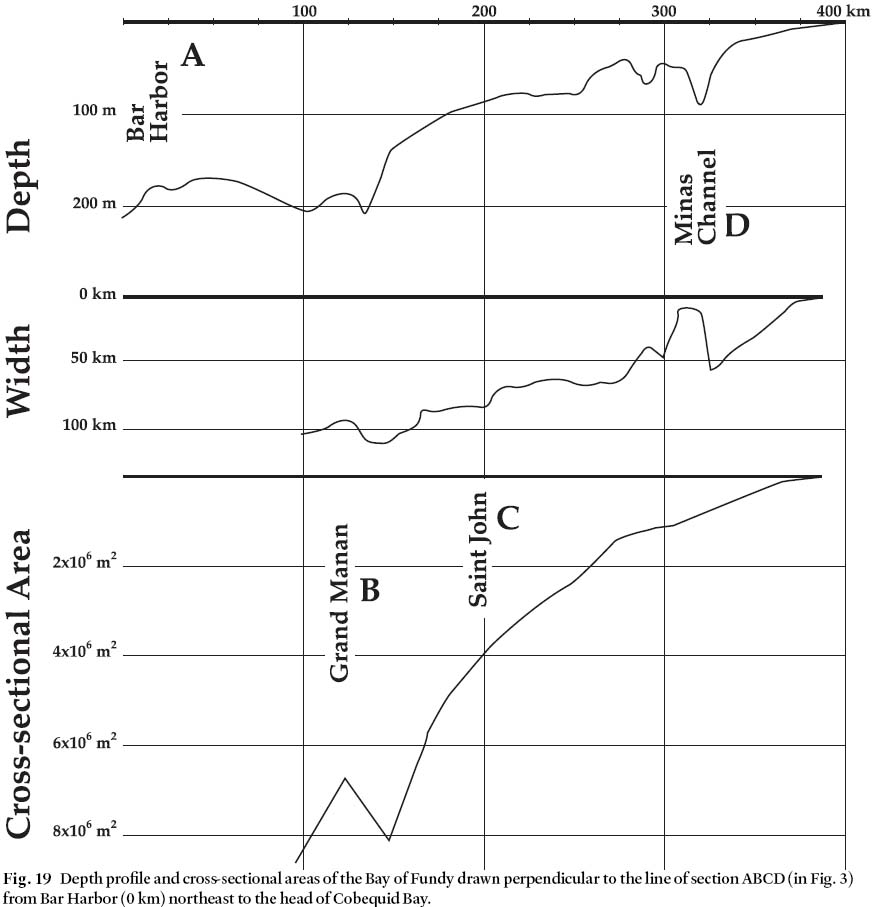
5.3.2. Exponential increase in tidal range and amplitude
136 According to tide tables published by the United States Department of Commerce (1953, 1975), the Bay of Fundy tops the list of those places where the largest tides are observed. In these tables Mean Range is defined as the difference in height between mean High Water and mean Low Water. The Spring Range is the average diurnal range occurring semi-monthly when there is either a full moon or a new moon. For some Canadian areas, data provided by Canadian tide tables are also noted. However, in these tables, the mean range is defined by the difference in height between the Higher (diurnal) High Water and Lower (diurnal) Low Water. A large range implies the difference between Higher High Water and Lower Low Water during exceptionally strong tides. Consequently, data in Canadian tide tables show greater mean and spring ranges than the U.S. tables.
137 In many estuaries and bays around the world the range of the tides increases exponentially with distance from any given reference point. This is the case in the Fundy - Georges Bank - Gulf of Maine system. Thus the range at a particular location Y2 can be estimated if the distance D (positive in the direction of the head of the Bay) from a reference station Y1 is known. If the percentage increase P per kilometre is known, the range T at point Y2 can be calculated with:

138 The importance of this relationship is illustrated for the Minas Basin. Note firstly (Table 3) that while the amplitudes of the semidiurnal tides increase toward Burntcoat Head at the head of the Bay and Basin, the diurnal amplitudes (DL) remain virtually constant at about 0.2 m. Nor is it likely that they will be altered when progressing into river estuaries. However, the semidiurnal tides are clearly a function of the distance from Saint John, where the principal tidal hydrographic station is located. This is shown in Table 14, where it is evident from the values of F (the exponential factor of the tidal increase over distance D) that the range of the semidiurnal tides increases as they advance into the Bay, at a rate P, of approximately 0.35% per km. This allows the local tidal range to be estimated rather accurately, with reference to the local Chart Datum, whence follow realistic estimates of Mean Water Level (MWL) and High Water level (HWL). Detailed examples of this procedure are documented in Gordon et al. (1985) and Desplanque and Mossman (1998a). The above relationship is relevant to issues as diverse as determining tidal boundaries (Desplanque and Mossman 1999a) and evaluating proposed tidal power generation schemes in the Bay of Fundy (Gordon and Dadswell 1984).
Table 14. Relationship between tidal magnitude and distance, the latter measured from Bar Harbor (Y 1), Maine
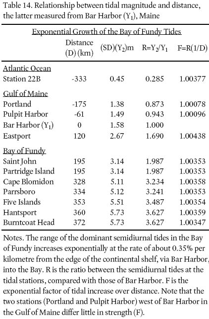
5.3.3. The importance of diurnal inequalities in the Bay
139 As noted earlier, strength of tides is mainly modified by changing distances between Earth and Moon, and because the Sun and Moon act individually from varying directions. Diurnal inequalities are due to changing declinations of the Moon and Sun with respect to the plane of the Earth's equator. The strongest diurnal inequality is possible when spring tides occur during the solstices when both celestial bodies are near their maximum declination, and acting together. As seen from Earth, the Sun appears to move through the plane of the ecliptic, which makes an angle of 23.452° with the Equator (see Fig. 6). The Sun is overhead at local midday at the Equator on 21 March and 23 September, and the length of the day and the night are the same everywhere on Earth. The Sun is said to have a north declination between the spring and fall equinoxes, and a south declination during the remainder of the year. It reaches its maximum north declination of 23.452° at the summer solstice in June (Fig. 6). The Moon goes through a shorter declinational cycle lasting 27.322 days. Also, because the Moon's orbital plane is at an angle of 5.145° to the ecliptic, its declination is more variable than that of the Sun. Thus the maximum declination of the Moon to the Earth's equatorial plane ranges from 28.597°N to 28.597°S 14 days later. Halfway through its nodical cycle, 9.3 years later, the range of the Moon's declination is reduced from 18.307°N to 18.307°S.
140 A sketch of the results of specific diurnal inequalities for locations in Maritime Canada serves to highlight details of the Fundy tides (Fig. 20). The combined effect of the semidiurnal constituents can be visualized as a wave, with nearly two cycles/ day moving through the area, whereas the combined diurnal constituents form a wave passing through a location once a day. If the High Water of the latter combines with one of the semidiurnal High Waters, the result will be an extra high tide (Schureman 1941). However the diurnal Low Water will then coincide with the next semidiurnal High Water, reducing it in strength. The two semidiurnal Low Waters will occur when the diurnal tide is at Mean Water Level, resulting in two Low Waters of equal height. This combination occurs in the Gulf of St. Lawrence, along the north shore of Prince Edward Island, and along the eastern shore of New Brunswick (Fig. 20, case 1). Here the two daily High Waters are unequal and the two Low Waters equal. When the Moon is close to the equatorial plane, High Waters are also equal for a day or so.
141 The reverse applies in the Northumberland Strait, where the High Waters are equal and the Low Waters unequal (Fig. 20, case 2). Here, one of the semidiurnal Low Waters coincides with the diurnal Low Water. In fact at times in sections of this area the semidiurnal tide is so weak that the amplitude of the diurnal wave is more than twice that of the semidiurnal amplitude. For example, in the western section of Northumberland Strait near Shediac Bay and Escuminac only one High Water and one Low Water may occur during the lunar day.
142 The situation concerning diurnal inequalities in the Bay of Fundy is detailed in Fig. 20, case 3. This illustrates a situation in which the midpoint of the falling diurnal wave coincides with one of the midpoints of a rising semidiurnal wave. The result is that a Lower High Water (LHW) is followed respectively by a Higher Low Water (HLW), a Higher High Water (HHW) and a Lower Low Water (LLW). Thus in the Bay of Fundy the sequence over a lunar day is typically HHW – LLW – LHW – HLW – HHW. The characteristic behaviour of the Fundy tides over the course of a month is shown in Fig. 21 for Herring Cove in Fundy National Park, N.B. Compared with marigrams from other localities in the Maritime Provinces, the diurnal inequalities of the Bay of Fundy are relatively modest.
Fig. 20 Sketch showing the combined effects of diurnal and semidiurnal tides for: Case 1 – Gulf of St. Lawrence, north of Prince Edward Island, and eastern shore of New Brunswick; Case 2 – Northumberland Strait; Case 3 – Bay of Fundy. Abbreviations: HHW = Higher High Water; ELW = Equal Low Water; LLW = Lower Low Water, etc.
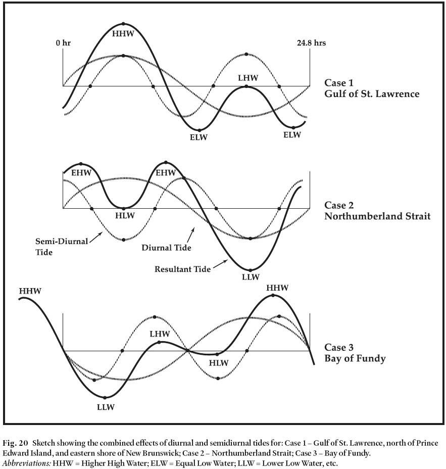
Display large image of Figure 20
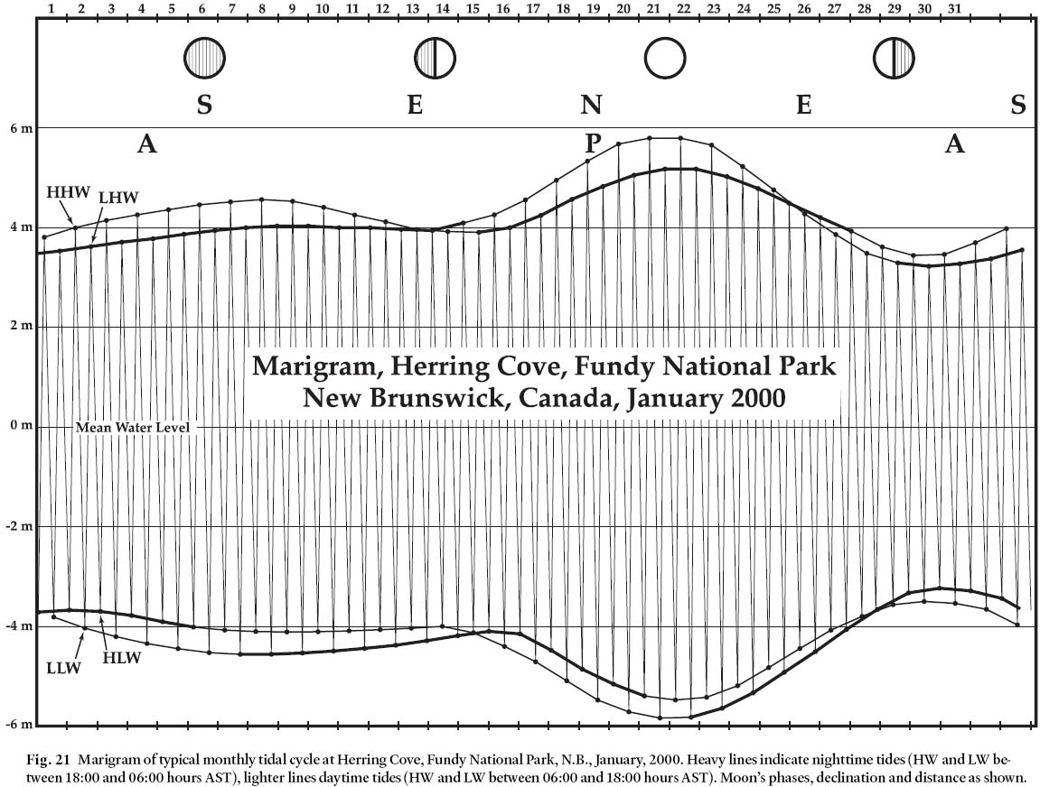
Display large image of Figure 21
143 Due to inertia in a frictionless system, the tides lag behind the forcing function by about 12 hours. For example, assume that at noon, 21 June, there is a solar (or lunar) eclipse (see Figs. 22A and 22B) over the Greenwich Meridian. At this time, in theory, the center of one "bulge" would be at, say 23.5°N, 0° longitude, the other at 23.5°S on the 180° meridian. In theory, the bulge should be over the Fundy area (65°W) around 16:00 hours GMT (i.e. about noon local time). However, observations in the Bay of Fundy will show that Higher High Water (HHW) on that day will occur at midnight (24:00 hours), and Higher Low Water (HLW) around 18:00 hours. The peak of diurnal inequality will occur around 21:00 hours, or about 9 hours later than the theoretical time (see also Desplanque and Mossman 2001b).
144 In contrast, during a solar (or lunar) eclipse on 23 December (Figs. 22c and 22d) a "bulge" would occur around midnight north of the Equator on the dark side of Earth. However, the peak of the diurnal tide would be around 9:00 hours, with HLW about 6:00 hours and HHW around noon. Thus in the Bay of Fundy, the HHW in spring and summer (i.e., between the equinoxes) occurs during the night time (6 pm. to 6 am.) and during the fall and winter (September to March) during the daytime. For the same reason Lower Low Water (LLW) occurs in spring and summer between midnight and noon (morning) and during fall and winter between noon and midnight (afternoon and evening). This situation results in a close coupling between tidal forces and biomass behaviour and production (Gordon et al. 1985) especially in the macrotidal conditions in the upper part of the Bay. It also plays an important role in determining sea surface temperatures (cf. Cabilio et al. 1997) and winter ice conditions in the Bay (Gordon and Desplanque 1983).
Fig. 22 Contrasts in diurnal inequalities developed in Bay of Fundy tides are greatest when spring tides occur during the solstices when Sun and Moon are near maximum declination and acting together (A to D); HHW = Higher High Water; LHW = Lower High Water. During the equinoxes there is little diurnal inequality and therefore Equal High Water (EHW) occurs day and night (E). Note: the declination of the Moon in June and December will not be exactly 23.5°, but anywhere between 18.5° and 28.5°.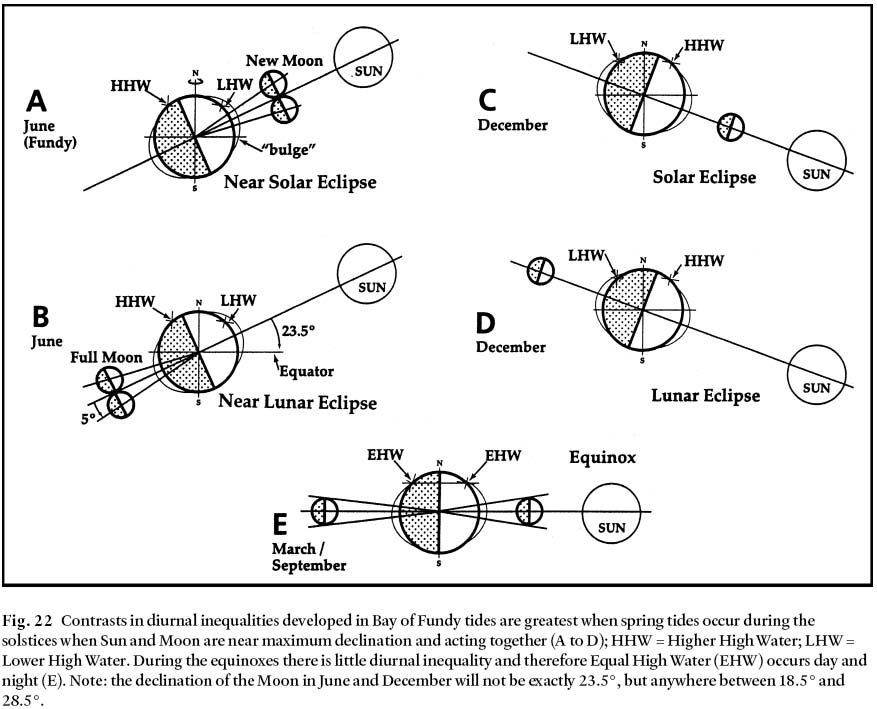
5.3.4. Tidal cycling at Herring Cove (Fundy National Park)
145 Tidal variations in the Bay of Fundy throughout the year are well illustrated by a typical annual record of tide levels at Herring Cove in Fundy National Park, N.B. The port of Saint John, 89 km more seaward, serves as reference port because the tides throughout the Bay of Fundy all show virtually the same features, except for the ranges of the local tides. The tide levels can be estimated from the tidal predictions for Saint John, N.B. (TSJ), as given in the Tide and Current Tables published annually by the Canadian Hydrographic Service (Canadian Tide and Current Tables 2004). The following equation is used to convert the given predicted levels of TSJ, measured in feet from the local Chart Datum (i.e. the lowest normal tide) to levels THC measured in metres from Mean Water Level at Herring Cove.

146 In the Bay of Fundy there is a close correspondence between the high tides predicted on the basis of astronomical conditions and those observed. The cyclic behaviour of the tides at Saint John, N.B. over a twenty year interval is shown in Fig. 23. The 206 day perigee/spring tide cycle is clearly evident, as are its matching cycles at 14 month, 4.5 yr and 18 yr intervals.
Fig. 23 Number of predicted (dotted areas) versus observed (areas enclosed by solid block) extreme High Waters per month at Saint John, N.B., for the interval 1947 to 1966. Cyclic behaviour of the tides is indicated by the 206 day perigee-spring tide cycles at 7 month (A to B), 14 month (A to B to C), 4.5 years (D to E, vertically), and 18 year intervals. Also shown is the number of tides that reached 28.0 feet (8.5 m) and higher, above Chart Datum. Note how the peaks shift 48 days (F to G – where the sloping lines cross the horizontal axis) to a later date each year.
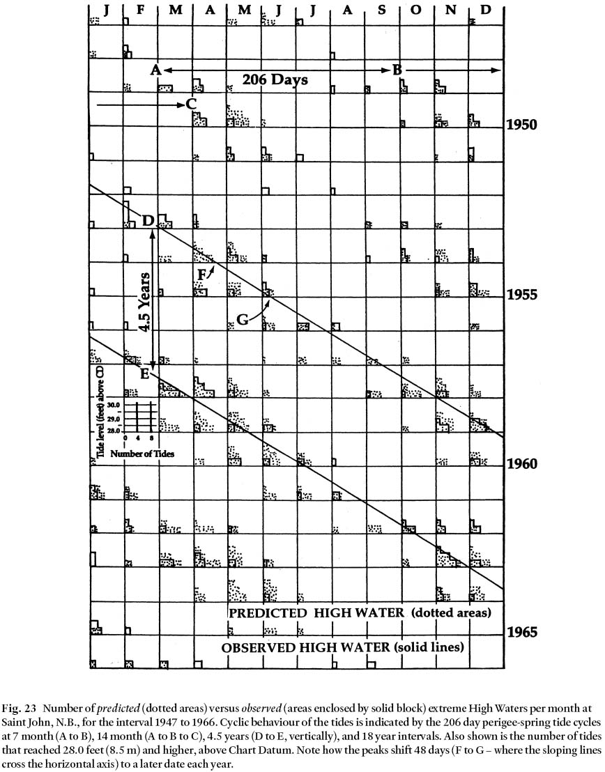
Display large image of Figure 23
147 It is instructive also to examine more closely the variations in tidal cycles over the course of one year at Herring Cove. For example, in 1988 (Fig. 24) there were 706 tidal cycles; on most days there are two High Waters and two Low Waters, being the highest and lowest levels predicted. The levels are measured from the Mean Water Level (MWL) that the water surface would assume if no tide-producing gravitational influences of Moon and Sun were present. Of course, if the combined gravitational influences of Moon and Sun remained constant, tidal fluctuations would also remain constant. However, influences of the Moon and Sun do not remain constant, neither in strength nor direction.
148 Since the angle of maximum declination of the Moon changes over a 18.6 year cycle, the situation depicted for Herring Cove in Fig. 24 will not be duplicated until 2005 A.D. In 1987, the Moon's declination reached its maximum value. On 6 December, 1987 the full moon was as high above the horizon as it could be. When the Moon is exactly above the Equator, as happens every 13.6 days, there will be no difference in strength of the two daily tides (no diurnal inequality). But the inequality soon reappears and will be strongest seven days later, when the Moon is either in its most northerly or southerly declination. At Herring Cove, this inequality results in differences in level reached by the daily tides of as much as 0.86 m for High Waters and 0.78 m for Low Waters. This occurred in January, July and December, 1988 (see Fig. 24); however, these differences disappear every two weeks as indicated where the HHW and LHW curves intersect, as do the LLW and HLW curves.
149 Because the new moon is never more than 5° different from the Sun's declination, there is a close relationship between the Sun's declination, the phase of new moon and its declination. Therefore the maximum diurnal inequality is centred around spring tides in June and December, and the weakest inequality during neap tides in March and September. When the perigean and spring tides coincide in June and December, the diurnal inequality causes one of the daily tides to be especially strong. This phenomenon, when combined with storm conditions, presents grave risks of destruction for property owners and settlements along the coastal zone (Taylor et al. 1996; Desplanque and Mossman 1999b).
150 One can expect stronger than usual tides a few days later than full and new moon, and weaker tides near the quarter phases of the moon. There is a certain inertia in the development of the tides analogous to the fact that, in the Northern Hemisphere, the months of July and August are on average warmer than June, when days are longer and the Sun is higher. Doubtless, friction is also an important constraint. For these reasons the highest tides occur a few days after the astronomical configurations that induce them.
151 Thus, as detailed in Fig. 24, perigean tides at Herring Cove in 1998 coincided with one of the month's set of spring tides around 19 February. Perigee occurred on 17 February at 11:00 AST, while the new moon occurred on the same day. One of the highest tides of the year (5.53 m+MWL) was expected with a delay of 48 hours shortly after noon on 19 February. On the same day the water was predicted to drop to its lowest level (5.87 m– MWL). On 25 April, when apogee coincided with a quarter phase of the moon, the water dropped shortly after midnight to 2.79 m below Mean Water Level. One might expect the lowest High Water levels near the days that apogee coincided with one of the quarter phases, as on 23 May or 1 December, when the water was expected to reach levels of 3.20 m+MWL. This is considerably higher than the predicted level of 2.70 m+MWL on 12 February, 12 March or 22 August, 1988. The explanation is that the first two dates were close to zero declination with nearly equal High Waters, while the latter three were close to maximum declination with 0.7 m diurnal inequality.
152 Note that two weeks before or after 19 February, the spring tides coinciding with full moon were not much higher than average tides. This is because the Moon was at apogee. This situation is repeated after about 6 and 7 months when, in September and October, the full moon occurs close to perigee. The 206-day cycle of perigean tides coincident with spring tides occurs all over the world, but it is far more pronounced (and far more important) in the Bay of Fundy because of the great tidal range. Two of these cycles last 412 days, meaning that each year the date that perigean tides are close to full moon is 47 days or about 1.5 months later on the calendar. This shift means that especially strong tides in the Bay of Fundy can occur during all seasons, depending on the year of observation.
Fig. 24 Chart shows predicted tidal movements throughout 1988 at Herring Cove, Fundy National Park, N.B. Solid lines indicate nighttim e tides (HW and LW between 18:00 and 06:00 AST). Daytime tides shown by dotted lines (HW and LW between 6:00 and 18:00 AST). Moon's distance, phases and declination, and Sun's declination are shown. Note ( KLMN) the coincidence of full moon and perigee just before the year's highest (and lowest) tides on 19 February. See text for details.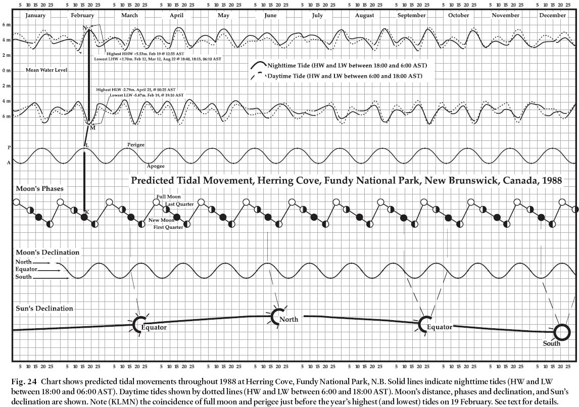
5.4. IMPACTS OF FUNDY TIDES
5.4.1. Erosion
153 The geological significance of the Bay of Fundy tides is most evident when linked to processes of erosion and sedimentation. A case in point is the effect of waves along some sections of the Fundy shore. Consider for example the shape of the curved erosional indentations in New Brunswick's rocky shoreline. Recall that throughout the Bay of Fundy the tidal range in absolute figures is high and that wave energy is concentrated near the surface of the water. One can also assume that the zone of the shoreline near the water surface will be most heavily subjected to wave action. Furthermore, during high water the foreshore is covered by a significant depth of water, and a much larger percentage of wave energy reaches the shoreline than when the tide is at low water.
154 Measurements of tidal levels conducted at Saint John, N.B. over an arbitrary 18 year interval are instructive (Figs. 25, 26, 27, 28). Note that the percentage of time (Fig. 28) that the tide water surface is in the upper or lower x% of the tidal range can be calculated for any tidal cycle, given that the amplitude ranges from 0 to 1 or, stated otherwise, from 0° to 90°. In the case of, say, the upper or lower 10% of the range, the amount of time is: [(arc sin 1 – arc sin 0.9) /90 · 100] = 28.7%. This figure contrasts with the percentage of time that the water surface spends in passing through the central 10% of the range. This later figure calculated as (arc sin 0.05 – arc sin 0.0) /90) · 100 · 2), amounts to only 6.4 % of the cycle. Fig. 28 (solid curve) shows clearly the focus of erosion exercised by tidal processes at Saint John upon a vertical profile of the shoreline over 18 years (Desplanque and Mossman 2001b).
155 A specific example is provided by "The Rocks", a tourist attraction at Hopewell Cape, N.B., just east of Fundy National Park (see Fig. 29). Here the continually sculpted erosion profile exactly reflects the total time that the water surface is situated at certain levels throughout all tide cycles (Desplanque and Mossman 1998a; c.f. Trenhaile et al. 1998). The profile corresponds of course only with the upper half of the "% Delta t" line indicated in Fig. 28, because the bottom half of the profile could not be formed due to the collected debris protecting the lower rocks from wave action.
156 Due to high tidal range, wave energy is thus expended over a considerable range of elevations, the highest being those in certain estuaries leading into the Bay. Using marigrams of various Bay of Fundy estuaries, we have documented the progressive reshaping of the tidal wave over its course and how its sediment-carrying and erosional capacities vary as a consequence of changing water surface gradients; likewise, how intertidal ice conditions contribute additional variations to an already complex tidal regime (Desplanque and Mossman 1998b). Clearly, Bay of Fundy tides play significant roles in a range of important geological processes centered on erosion and sedimentation and bearing directly on coastal construction/installations, dredging, dam and causeway construction, fishing etc. (Daborn and Dadswell 1988; Thurston 1990; Percy et al. 1996).
Fig. 25 Profiles across the range of average: large tides, mean tides, and small tides, as recorded at Saint John, N.B., (1947– 1964) give the percentage of time that the water surface is located at a particular elevation during different tides (MSL = 14.36 feet + CD). Compare with Figs. 26 and 27.
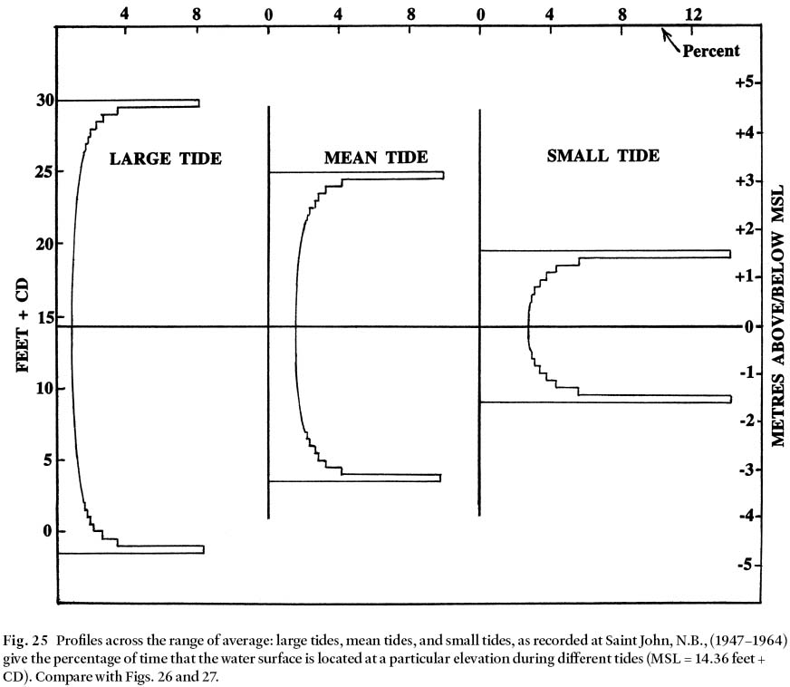
Display large image of Figure 25
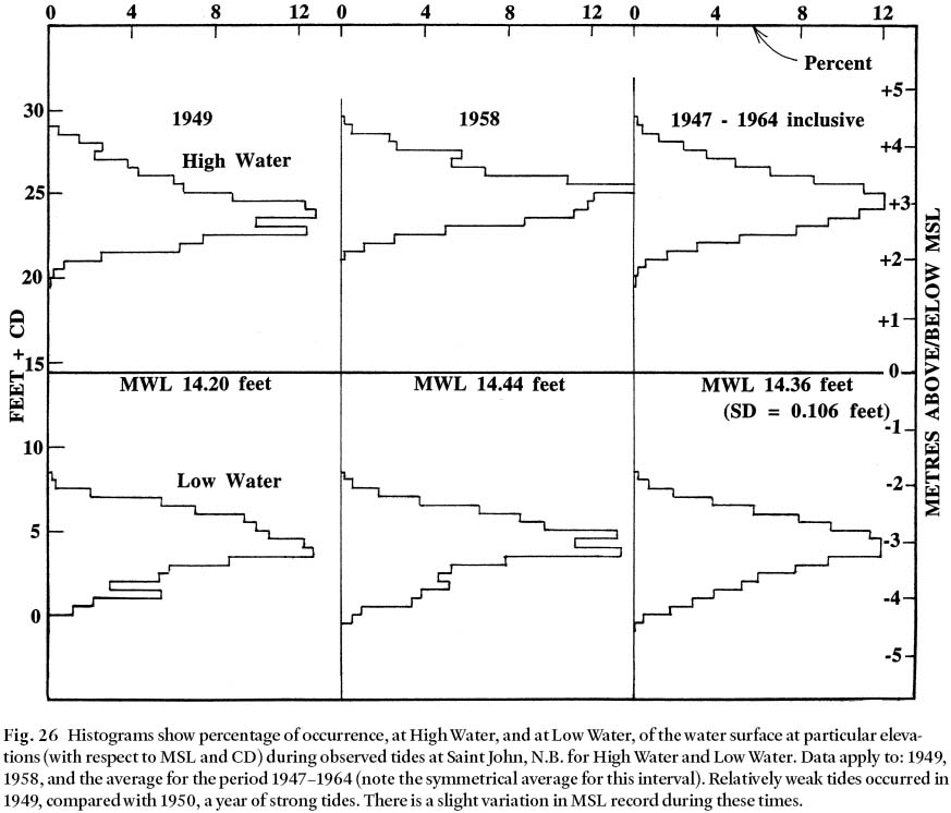
Display large image of Figure 26
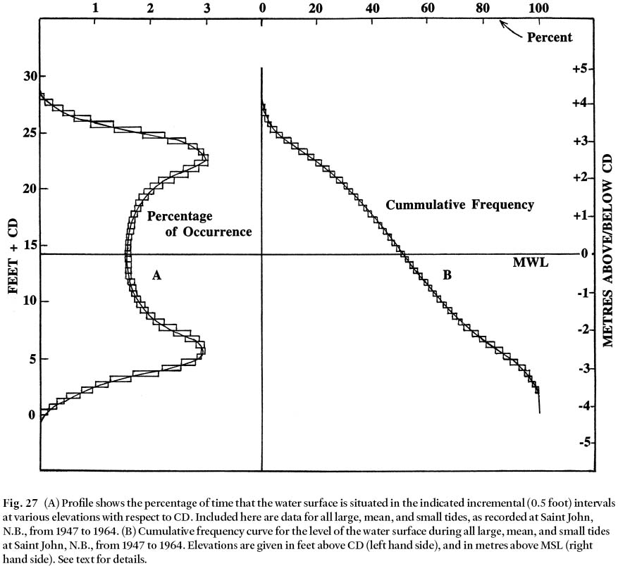
Display large image of Figure 27
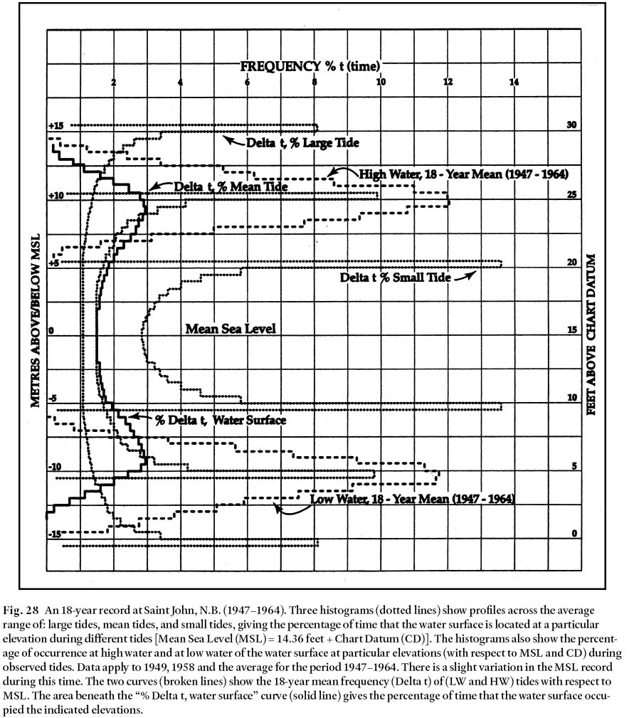
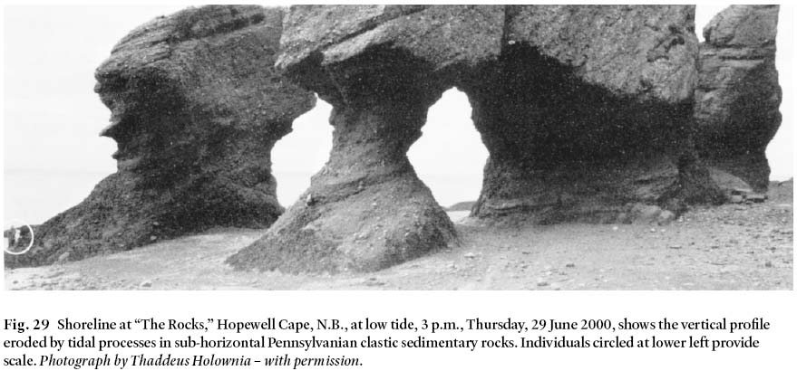
5.4.2. Sedimentation and related processes
157 Current regimes are critical to sediment dynamics and have significant scientific and economic applications, especially in the area of environmental marine geology. The results of the pioneering work of Pelletier (1974) in the Bay of Fundy suggest that major pulses of hydrodynamic energy are reflected in the coarse-grained sedimentary material concentrates as transverse bands across the central portion of the Bay and at the extreme eastern and western approaches. Pelletier (1974, p. 92) considered it likely that tidal velocities dominate over residual current velocities, and that interaction with the sea floor would produce a "wash-board" pattern of sediment distribution. His conclusions are elegantly complemented by the results of recent work by Fader (1996), who assessed surficial sediment stratigraphy, aggregate resources, and seabed dynamics of the inner Bay of Fundy using a new multibeam bathymetric mapping system. Fader (1996) shows the presence of extensive areas of thin gravel lag overlying thick glaciomarine sediments. Overlying the gravel are large transverse fields of active sand bedforms, likely formed by winnowing processes initiated by increases in tidal range about 8000 years BP. The numerous symmetrical sand waves range in length from 0.3 to 0.8 km and are oriented normal to the length of the Bay.
158 Fader's interpretation of the bedforms and related processes suggests that the large sand waves are presently inducing scour of the adjacent seabed by virtue of their presence, size and redirection of flow. This localized scour has coalesced in some areas, resulting in major erosion and deepening of the seabed of up to 10 m. The result is the release of large quantities of glacial mud to the water column, leaving behind residual sand deposits (cf. Amos and Joice 1977). Input of this subsea glacial age mud was not previously accounted for in the determination of sediment budgets. It could explain recent increasing mud content and textural alterations on mud flats in the upper Bay of Fundy, which has important implications for the survivability of migratory bird populations (e.g., Shepherd et al. 1995). Indeed, scour of the seabed with localized over-deepening could also explain observations by the fishing community of changing bathymetry. Perhaps more importantly, the apparently active and increasing erosion of the seabed could signal that the Bay of Fundy is experiencing a level of dynamics never before observed. At present, models of resonance length are too coarse to validate these observations, but there seem to be important connections between tides, currents, sedimentation, erosion, and the biological community. Implications of these findings have yet to be applied to seabed fishery management practices.
6. Tidal Bores in Estuaries (TOP)
6.1. TIDAL VOLUMES, TIDAL PRISMS
159 Tidal waves, as recorded on marigrams, are typically symmetrical, the shape of the falling limb being the mirror image of the rising limb. However a process of translation takes place as a tidal wave enters a shallow estuary. The wave becomes distorted (see equation 7), the rising limb being compacted within a shorter period, whereas the period of the falling tidal wave increases (Carter 1998). Friction is often given as the cause, although this is not necessarily so. This is because the rising tide is a function of the predetermined tidal wave, whereas the return is a matter of hydraulics peculiar to that particular channel. We define a tidal river as that stretch of a freshwater river where the dominating factor in shaping the river channel is the freshwater regime. A tidal estuary is the mouth of a tidal river where the tidal flow regime shapes the channel bed. Because tidal range and freshwater flow are variables, the tidal river and the tidal estuary are separated by a transitional section where the dominance of tidal regime and freshwater regime alternate.
160 The volume of an estuary upstream of an arbitrarily chosen cross-section can be conveniently divided into two parts. The tidal prism is the top part of the estuary between the Low Water and the High Water levels. More simply it is the volume of water flowing in and out of the estuary with the rise and fall of the tide. The tidal volume is that portion below Low Water Level. Because tides are variable in strength, the tidal prism and the tidal volume are variable, as is the wet cross-sectional area through which the water that fills the tidal prism must flow. In general, where a moderate tidal range prevails in combination with deep waters and a limited surface area, only small currents are required in the estuary to have its tide follow the outside tide in terms of vertical movement. An increase in the current speed can only happen when the water surface drops in the direction of flow. In outside tidal waters, the current speed is generally so small that it can be neglected. During Low Water, the upper parts of an estuary may become virtually empty. Water levels in the estuary are only able to match the rising tide if enough water flows through the available cross-sectional area to fill the tidal prism to the level reached by the tide. Except for the extremely critical conditions of tidal bore development, the maximum current speed possible in a cross-sectional area is limited, being proportional to the square root of the water depth. Rectangular cross-sectional areas are able to discharge much more water than either parabolic or triangular cross-sectional areas. Sediment transport is of course associated with the tidal cycle, and at any given location velocity changes in tidal currents bring about periodic changes during flood and ebb portions of the cycle.
161 The vertical movement Y of the tide in seas and deep bays can be roughly expressed as:

162 An appropriate speed number (n) for describing average semidiurnal tidal conditions in the Bay is 28.984° per hour or 1.405 · 10 – 4 radians per second. The reciprocal v, of the last value is 7116.5. When seconds are used as time units, (22) can be replaced by:


163 However, there are conditions in which the rate p' cannot equal Y', either because the values of Vm and A are relatively small compared to S, or because the value Vm depends on the depth of the flowing water. In order for the incoming tide to gain speed, the water level of the tidal volume must be below the level of the outside water. If the wet cross-sectional area is A, the required velocity V through the gap must be at least Y' · (S/A) ms -1, because eddies and local currents prevent the total area being available for the discharge. These relationships are explored in greater detail in section 6.3.
6.2. WAVES OF TRANSLATION – TIDAL BORES
164 Basically, a tidal bore is a wave of translation, a hydraulic shock wave formed by a rolling wall of water. Analogous to a sonic boom (Lynch 1982), it develops when the rising tide forces water to move up a river channel faster than it otherwise could propagate in a given depth of water. Ideally the tidal range should be high, the river shallow, and the channel gradient slight. In reality a tidal bore is a single wave or a group of symmetrical sine waves that travel upstream signalling the turn of the tide at Low Water. In deep water these waves move at different speeds and separate from each other. However, in shallow water the component waves of the bore are translated into a single wall of water.
165 An estuary generates a bore when the level of the water surface is unable to keep up with the rising tide. Too small a cross-sectional area is available in the river channel. Thus at the mouth of the estuary more water enters than can be moved along at the front of the bore. The developing wave travels more quickly in deep water than in the shallow water of the estuary. Upstream, cross-sectional area and depth decrease. Consequently, possible current speeds are smaller in front of the advancing wave and the volume of the flow is decreased. As excess water overtakes the bore its height increases. Bore height continues to rise until the rate of rise in the tide becomes insignificant. The bore terminates when the tide reaches its most upstream point in the estuary. Under favourable geographical and astronomical conditions, a bore may be a metres-high wall of water moving up an estuary with a roar heard tens of kilometres distant; under other conditions, it is a leisurely moving ripple.
166 Waves of translation are surprisingly common. For example, during a heavy rainfall a sheet of water may be seen flowing down a steeply-sloping asphalt street. Here at regular intervals, waves form which move faster the higher they become. Another example occurs with the last uprush of water upon a sandy beach, pushing bits of shell, seaweed and other light materials to the line of its farthest reach. Here it is momentum that carries the water up the beach and over a slope upon which water from the previous wave has mostly been drained. The steep front of the breaking wave is, in effect, the crest of a miniature bore. These waves also occur in canals used for inland navigation when water is suddenly discharged from a reservoir or lock into the canal. Wave height here depends on the amount discharged and the dimensions of the canal. However, this is a negative wave of translation that results in a distinct drop in the level of water moving down a canal. Likewise, a negative bore also may occur when a lock is filled at an appreciable rate. The following theory outlines the conditions governing maximum flow.
6.3. LIMITING CONDITIONS FOR BORE DEVELOPMENT
167 Elementary physics provides the following equations for free fall near the surface of the Earth.
g = the acceleration (9.806 ms
-2) due to the gravitation of the
Earth near its surface.
h = 0.5 g · t
2
h = vertical drop in free fall
v = g · t, the speed attained after at the end of a vertical drop
t = time
Thus:

168 Note that this relationship between drop and velocity holds whether the resulting movement is vertical or not. Pressure due
to differences in surface elevations will cause the same speeds. Also,
Q = c · v · A , where Q = volume of water passing through the channel in 1 s and
c = coefficient of loss in average speed due to eddying and heat production,
v = theoretical speed = (2g · h)
0.5
A = wetted cross-sectional area of channel, and
D = water depth.
169 Assume that water is moving from a deep reservoir under the conditions illustrated in Fig. 30. In order to attain a speed v, the surface of the water near the entrance has to drop h metres, causing a pressure on the water in the cross-sectional area equal to the weight of the water in the column h metres high. In a rectangular channel B metres wide (Fig. 30) and the water D metres (H – h) deep.

Q will be zero if h = 0 (No speed)
Q will be zero if h = H = 0 (No area)
Q will be maximum when dQ = 0 0.5
Fig. 30 Sketch illustrates the condition of maximum flow in a rectangular channel caused by a decrease in head (h) of waterin a reservoir feeding into a channel H m below surface of the water reservoir. The limits for the ratio d/H for rectangular, triangular, and parabolic channels respectively, are 0.667, 0.80 and 0.75. For trapezoidal receiving channels, the limit is variable, but somewhere between these limits.
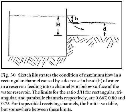
Display large image of Figure 30


170 In a sinusoidal tidal movement the height of the tide can be expressed as:


171 In order to establish the dimensions of discharge sluices in major Bay of Fundy estuaries, it was necessary for the MMRA to determine the volume P of the tidal prism upstream of the construction sites. Following surveys it was found that there was a rather constant relationship between the tidal cross-section A and the volumes P of the tidal prisms upstream of them. A general relationship for estuaries or tidal basins has been proposed by Jarrett (1976) and by Van de Kreeke (1998). Regional characteristics determine the constant and the power of A. This relationship can be empirically expressed as:

172 Tidal estuaries where bores occur are flat bottomed and the width is large compared with the possible water depth. Thus the cross-section is close to rectangular in shape. The following discussion assumes a rectangular cross-section. Thus A = B · D.
173 Taking d(h) as zero, so that the volume of a rectangular tidal prism to be filled in 1 second becomes:


174 Note that the critical depth does not change much when the tide is near mean sea level. Thus the simplification of neglecting d(h) /dt has no serious effects. Note too that the critical bottom elevation is at lower elevations when the channel is wider. Therefore the bore can start as soon as these conditions are met.
175 As not enough water can enter to raise the water levels at the same rate as the tidal waters, the water that is able to enter the estuary will flow at the maximum speed, depending on the depth of the water. The first water to enter flows considerably slower than that which follows, as depth increases. In fact the later water will overtake the earlier water, with the result that the wave entering the estuary will do so as a bore of increased height. The water in the bore front is thus a mixture of volumes of water that had different initial speeds and momentum. For this reason the speed Vb of the bore is likely to be somewhat less than maximum flow speed indicated by the height H of the bore. Thus:

176 Note that the maximum flow condition is actually unstable, although depths can deviate slightly from the critical depth without changing the discharge very much. This could explain the presence of "whelps" behind the bore front. Whelps are waves that are very conspicuous after the passage of the bore. But even if maximum flow conditions are not reached, the water surface elevation in the estuary will always be lower than the rising water in the tidal sea. This is because of the required velocity heads. Thus water near the head of the estuary will be flowing on a slope with decreasing cross-sectional area. Consequently the sinusoidal wave is distorted and becomes less and less symmetrical. This can be illustrated by plotting the centre line in marigrams, obtained at different locations along the estuary (see section 7.2).
177 A bore will be formed if the frontal part of the distorted tidal wave becomes vertical. It will grow in size when it flows over horizontal bottom plain(s). However, if the elevation of the estuary bottom is rising steeply, there is less chance of a large bore due to inadequate distance and time. When a tidal bore flows over a dry tidal flat, or shallow water, its progress is unrestricted. But as soon as the original water depth is 2/3 or more of the water depth of the bore, maximum flow conditions no longer prevail and progress becomes restricted. This figure approaches the 1.4 ratio, evidently the dividing condition between breaking and non-breaking bores. Note that in parabolic-shaped channels the original water depth would interfere when 3/4 of the bore depth, a figure corresponding with a ratio of 1.33.
178 With the exception of the Bay of Fundy, tides along the coastlines of North America are not particularly strong and thus not conducive to the formation of tidal bores. However, the bottom gradients of the Bay of Fundy are too steep to permit a large bore to develop. Thus, a tide with an amplitude of 5 m can only develop a bore 0.6 m high after travelling 6.2 km over a horizontal plane. With a tide of 2.6 m amplitude it requires a distance of 12 km, and with an amplitude of 1.5 m, a distance of 21 km is needed in order to develop a 0.6 m high bore. No bore will form with a tide of 5 m amplitude if the estuary gradient is steeper than 0.000193. A tide of 2.6 m amplitude cannot form a bore in a channel with a gradient more than 0.0001. In short, channels of certain dimensions can discharge quantities of water up to a certain limit, at which point maximum flow conditions prevail.
Table 15. Data for two hypothetical river channels illustrate conditions favouring tidal bore formation
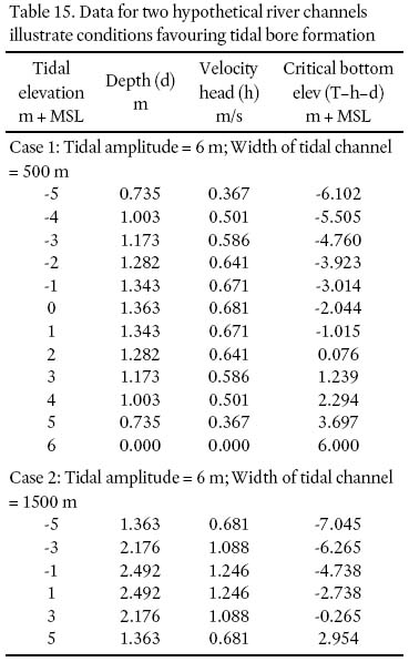
6.4. TIDAL BORES IN THE BAY OF FUNDY
179 The global catalogue of tidal bores (Bartsch-Winkler and Lynch 1989) includes five of the main bores from the Maritime Provinces, all in the Bay of Fundy area. These are in the Hebert, Maccan, Salmon and Shubenacadie rivers (Nova Scotia) and in the Petitcodiac River (N.B.). Each constitutes an important tourist attraction at several localities. The rivers Hebert and Maccan empty into Cumberland Basin upstream from Fort Beausejour. Like all Fundy examples, the height of bores developed in these two rivers is variable, being dependent upon predictable astronomical conditions. The chief controlling factor is the rate of rise of water in Cumberland Basin, which of course peaks during either the new moon or the full moon phase, whichever is closest to perigee. Compared to predicted arrival times of tides using Saint John tidal data, the arrival time of the bores in these two rivers is generally earlier at spring tides than at neap tides. The same is true of the Shubenacadie and Salmon River bores near the head of the Minas Basin.
180 In contrast to the Hebert, Maccan, and Salmon rivers, the (observed) arrival times of the bore in the Petitcodiac River at Moncton is delayed more at spring tides than at neap tides. A check on the difference between predicted and observed tides at Saint John, and the prevalent weather conditions at the time, rules out weather as a cause of the delay. The explanation may lie in the fact that the Petitcodiac River bottom is below mean sea level, whereas at the other localities, river bottoms are well above mean sea level.
181 Unfortunately, a causeway built in 1968 upstream from Moncton shortened the estuary by about 21 km and decreased its tidal prism by about 20 · 10 6 m 3. A similar story applies to numerous estuaries: when estuary equilibrium is disturbed, channel readjustment follows. In the Petitcodiac, the decreased outgoing tidal flow was no longer able to remove as much silt as previously (Thurston 1990). Consequently the channel lost 450 m of its width and the bottom gradient became steeper because of a tremendously increased rate of silt accumulation. For example, between 1968 and 1971, an estimated 10 · 10 6 m 3 of sediment accumulated in the estuary.
182 Change in shape of the channel has greatly affected the size of the bore (Figs. 31, 32), which now must follow a steeper, more tortuous channel. As a result the bore falls far short of the 1.2 m height that it had prior to causeway construction. Further, the arrival time of this tidal bore has also changed during the last several decades. In 1920 Dr. W. Bell Dawson determined that the Petitcodiac bore occurred 2 hours and 22 minutes before High Water (spring tide) in Saint John. The present daytime difference between the arrival of the bore and Saint John High Water of 1 hour and 38 minutes indicates that the causeway and resultant change in the shape of the Petitcodiac River estuary has retarded the arrival of the bore by almost one hour since 1920. (The Bell Dawson difference was used and mentioned as a footnote in the tide tables between 1922 and 1983 inclusive. In the 1984 tables a shift was made to the new difference of 1 hour and 38 minutes).
Fig. 31 Tidal bore on the Petitcodiac River, viewed (ca. 1964) from the old Irving Oil dock in Dieppe, N.B. This bore started to develop at Stony Creek near Dover, 10 km downstream from Moncton/Dieppe, and 17.5 km upstream from Dorchester Cape. Photograph New Brunswick Provincial Archives. Photograph by David Coon, Conservation Council of New Brunswick – with permission. Fig. 32 Cross-section of the Petitcodiac tidal bore at Moncton, N.B. determined by measurement of water height with passage of time. Note the 2-foot (0.61 m) high steep front of the bore, the relatively rapid rise to 3-feet (0.91 m) and the further 6-foot (1.83 m) rise during the next 20 minutes. Modified after Clancy (1969, p. 120).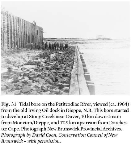
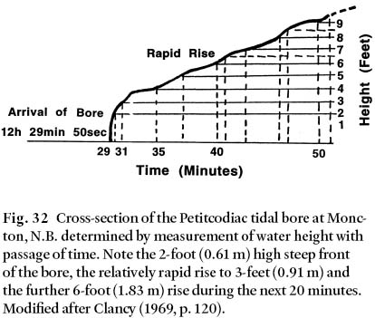
6.5. QUIANTANG RIVER BORE, CHINA
183 The decline of the Petitcodiac bore disappoints local tourists and tourism promoters alike. In curious contrast, in China there is an ambitious program to suppress the bore in the Quiantang River. This bore and those of the Amazon delta (McIntyre 1972) are among of the most spectacular in the world. In the case of the Quiantang River, the drainage area is about 50 000 km 2 2(roughly equivalent to the watershed of the Saint John River, N.B.). Its tidal section starts at Fuyang, which is occasionally reached by a bore. However, the estuarine portion commences 18 km downstream of Fuyang, at Wenjiayan, and continues 101 km further downstream to Ganpu (Fig. 33). The main tidal channel shifts frequently, sometimes 245 m a day. Near Hanghzou the width of the estuary is about 1 km, and 20 km at Ganpu. Beside the tidal channels are vast tidal flats raised to about 1.2 m below the highest tide levels. During low tide the channel is shallow, many sections having a depth of 1 to 2 m, but even here where flow is rapid, ships of 100 tonnes or less can navigate.
Fig. 33 Map of Qiantang River estuary near Hangzhou, China. After Dai Zeheng (1982, p. 2).
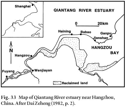
Display large image of Figure 33
184 Beyond Ganpu is the flaring Hangzou Bay, which runs 100 km to its 95 km wide mouth, open to the East China Sea. The tidal range in Hangzhou Bay doubles over this distance of 100 km to a maximum range of 8.93 m at Ganpu. This rate of increase is 0.7% per kilometre, twice the rate of the Bay of Fundy. Upstream from Ganpu, the river bed rises abruptly and the channel becomes shallow. According to Dai Zeheng (1982), the bore begins to form near Jianshan 19 km upstream from Ganpu, and reaches its maximum height in the vicinity of Baboa (33 km) and Haining (40 km) (see Figs. 34 and 35). The height of the bore is normally 1 to 2 m, but reaches a maximum height of 3 m. It usually travels 5– 7 ms -1 (18– 25 km/hr) but has been recorded at 12 ms -1 (43 km/hr) (van der Oord 1951). Stretched across the 3 to 10 km wide channel, it moves upriver like a silver curtain with a roar that can be heard over a distance of 20 km.
185 Although there are few accounts of the Qiantang bore in western literature (see Darwin 1898), the bore must have been present in the river for at least the last 1000 years. Long standing doubts of its existence probably arose because Marco Polo never mentioned the bore in his detailed account of the city of Hangzhou (which he called Kinsai). According to Masefield (1926), Marco Polo probably left this tale untold lest he lose all credibility. Unfortunately the original manuscript is lost, and the oldest written account of his story dates from 1559. The tale of a metres-high wall of water entering the river at regular intervals was probably demanding too much from his audience.
Fig. 34 The "crossing bore" at Babao, Haining, China, 1975. For scale, note the person standing on the wall (left side of photo). Photograph by Dai Zeheng – with permission. Fig. 35 The tidal curve of the "crossing bore", also known as the "rolling thunder" and the "wet wild beast". LW = low water. From Dai Zeheng (1982, p. 3), with permission.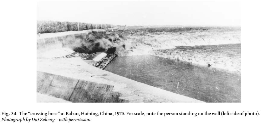
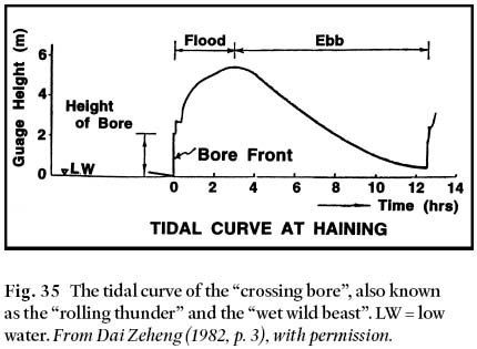
7. Ebb and Flow in Estuaries (TOP)
7.1. INTRODUCTION
186 Because tides are variable in strength, the tidal prism and tidal volume in an estuary are also variable as is the wet cross-sectional area, which is that part of the total cross-sectional area filled with water. As discussed in section 6.3, it is through this wet area that the water which fills the tidal prism must flow. The upper parts of an estuary may become virtually empty during Low Water. Water levels in the estuary are only able to match the rising tide if enough water flows through the available cross-sectional area to fill the tidal prism to the level reached by the tide (Lauff 1967; Carter 1998). In many cases this is physically impossible as the maximum current speed possible in a cross-sectional area is limited, being proportional to the square root of the water depth (Kjerfve 1988). Rectangular cross-sectional areas are able to discharge much more water than either parabolic or triangular cross-sectional areas because the larger cross-sections allow higher current velocities.
187 In channels that empty, or nearly empty, during Low Water, the first water to return after the turn of the tide is very much restricted moving into the estuary. This is so even discounting friction, because the water depth and cross-sectional area are very small or zero. However the following water finds a partly filled channel and can thus move faster and at a greater discharge rate. As long as the discharge is inadequate to fill the tidal prism at the same rate of rise of water surface as the outside water, the result is that the seaward gradient of the incoming water will initially have a strong upward curvature. This curvature may become so strong that a bore will form at the bottom of the incoming wave.
188 What happens when, at a certain location in the estuary, the water reaches its highest level? Certainly the more upstream parts of the estuary remain unfilled with water. Seaward of this point the water level is already falling. Thus water continues moving landward on its own inertia when the high tide level is reached at that point. As a result, the water surface has already dropped before the direction of flow reverses. Thus the time of peak elevation and zero velocity are not coincident. When the water ceases its advance into the estuary it has already a considerable downward slope seaward. Soon a sizable seaward current develops, occupying a smaller cross-sectional area than when it moved into the estuary on the rising tide. The falling water level may at first follow the outside tide rather well because of the large cross-sectional areas, but progressively the reduced depth restricts water outflow. Consequently the seaward gradient of the water surface during ebb flow now has a downward curvature.
189 In terms of sediment transport this means that while the incoming tide is at high levels and gradually reducing in speed, its sediment carrying capacity is reduced (Amos and Tee 1989; Amos 1995a). Much of the released sediment is spread over the full height of the channel banks, and during very high tides, over the salt marshes also (Postma 1967). However the outgoing tide is concentrated toward the bottom of the channel, having at times higher speeds than the incoming tide. This situation promotes erosion through undercutting of the channel banks. Excess material high on the banks will slide down, resulting in unstable soil conditions. In testimony, the banks of tidal creeks and rivers in the Bay of Fundy region are characteristically bare of any vegetation except perhaps for some being transported downslope by undercutting (Scott 1980). Only where currents are slight is vegetation able to take root. Overall the intertidal flats of estuaries may vary seasonally, storing clays and silts during summers and removing them during heavy freshwater run-offs.
7.2. RESHAPING THE TIDAL WAVE THROUGH TIME
7.2.1. The Shubenacadie estuary
190 When the tidal wave enters a shallow estuary its sinusoidal symmetry becomes distorted. The rising limb of the curve becomes compacted within a shorter period, whereas the period of the falling tidal wave increases. The manner in which a tidal wave may be reshaped as it moves into an estuary is well illustrated by conditions in the Shubenacadie and Cornwallis river estuaries in Nova Scotia (for locations see Figs 3 and 43). At the mouth of the Shubenacadie estuary the rising tide is retarded by the shallow waters of Cobequid Bay (see Fig. 36). However, the centreline (CL1), being the locus halfway between rising and falling tide levels at Black Rock at the mouth of the river, is almost straight and vertical in the uppermost part of the marigram. This means that there is little distortion in the symmetrical shape of the local tide wave. The near-vertical rise of the tide at the bottom of the incoming tide wave (K) indicates that a bore may possibly develop.
191 The curvature (asymmetry) of the centre lines at locations further upstream indicates that the tidal wave is becoming increasingly distorted with much steeper rises of the tide, and slower rates of drop. Meanwhile, the thalweg (the median line of the channel) of the estuary is rising at some distance beneath points K, L, M, N, and O (which indicate the water level in the river before the tide wave arrives), thus increasingly limiting the inflow of tidal water. The High Water levels rise for about the first 8.3 km (A to B in Fig. 36) before gradually dropping (B to E). This situation is reflected by the asymmetry of the marigrams, as indicated by the increasing curvatures of their centrelines (CL1 to CL5) with distance from the river mouth. Eventually, the water levels in the river will fall back to K, L, M, N and O, as the water exits the estuary prior to the next incoming tide.
Fig. 36 Curves 1 through 5 indicate modifications to the shape of the tidal wave based on measurements of the whole marigram, at various cross-sections of the Shubenacadie River, near Truro, N.S., on 15 October, 1970: 1) Black Rock, at mouth of the river, 0 mi (0 km); 2) D.A.R. (Dominion Atlantic Railway, precursor to the Canadian Pacific Railway) bridge, 5.3 mi (8.53 km) upstream; 3) Fort Ellis - Stewiacke River, 14.7 mi (23.65 km) upstream; 4) Shubenacadie high water bridge, 20 mi (32.18 km) upstream; and 5) mouth of Gays River, 24 mi (38.62 km) from the Shubenacadie River's mouth. Saint John tide was 27.9 ft (8.5 m) plus Chart Datum at 11.30 AST. CL is the centreline of the tidal wave and the high water levels are A, B, C, D, and E. The points K, L, M, N, and O indicate the initial freshwater level at the location (e.g., K = Black Rock) at the time (in hours) indicated.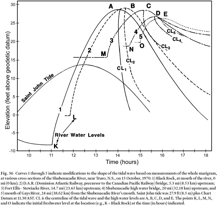
7.2.2. The Cornwallis River estuary
192 Figure 37 shows the reshaping of the tidal curve in the uppermost 4 m, near the peak of the tide, for a tidal wave in the Cornwallis River, N.S. The asymmetry of the marigrams, and the shape of the centrelines (CL1, etc.,) show that the further the wave goes into the estuary (Site #1 to Site #5), the slower the rate of rise of tide near the peak (A, B, etc., on Fig. 37) and the faster the drop after the peak has passed. Initially, the curvature of the centrelines is reversed near the top of the wave (eg., A), but further upstream (eg., D) this reversal disappears.
Fig. 37 Observed tidal curves at five stations, illustrating modifications to the shape of the top of the tidal wave in the Cornwallis River, near Kentville, N.S., on 5 September, 1956. Station 1, (Port Williams bridge), 0 km upstream; Station 2, 2 mi (3.2 km) upstream; Station 3, 6 mi (9.75 km) upstream; Station 4, 8 mi (13.1 km) upstream; Station 5, 9 mi (14.3 km) upstream. High Water on the Saint John River at 27.4 ft (8.4 m) above CD at 11.43 AST. Data drawn from MMRA observations. The five axes indicate the "centreline" or loci halfway between the rising and falling tide levels; measurements apply here only to the uppermost 4 m of the tidal wave.

Display large image of Figure 37
193 Figure 38 shows the momentary gradients of the water surfaces at different times during the passage of the top of the Cornwallis River tidal wave. While the wave is moving upstream on its own inertia through this section (between 12:15 and 13:30 hours), the gradients of the water surface seaward of the wave top are negative and rather uniform. The moment its inertia is spent, the water starts moving backward toward the sea. The difference is that now, on the outflow, the gradients are not only reversed but are steeper because water levels have dropped considerably, forcing flow through small cross-sections at higher velocities. Note too that the water's surface is curved downward, concentrating the flow of outgoing water in the lower section of the channel.
Fig. 38 Observed water surface gradients at different stages on the Cornwallis River, Nova Scotia, using measurements taken only near the peak of the tide, on 5 September, 1956. (Times tie in with those shown in Fig. 36). Note the relatively uniform gradient of the water surface of the rising water (time 12:15 to 13:15) compared with the progressively steeper gradient during reversed flow in the channel. Locations: #1, 0 mi (0 km) mouth of the Cornwallis River; #2, 2 mi (3.22 km) upstream; #3, 6 mi (9.65 km) upstream; #4, 8 mi (12.87 km) upstream; #5, 9 mi (14.48 km) upstream. High water on the Saint John River was 27.4 ft + CD at 11.43 AST.

Display large image of Figure 38
194 The difference between tidal rivers and tidal creeks is that tidal rivers discharge fresh water from upland watersheds. In the upper reaches of the estuary, freshwater flow maintains a drainage channel, the size of which is related to the river discharges. In contrast, a tidal creek is formed by tidal water that moves onto a tidal marsh during Higher High Waters, discharging following the turn of the tide. The only fresh water moving in such creeks is rain water collected on the salt marsh itself. In effect, creek formation requires a certain area of marsh because the erosion process demands a minimum flow volume from the marsh in order to initiate channel cutting through vegetated soil. For this reason there always exists a margin of land not cut by tidal creeks on the seaward side of dykes built on reclaimed salt marshes. This feature is readily visible on aerial photographs of out-to-sea marshes.
195 Tidal channels reach a quasi-equilibrium condition ranging between certain limits. In spring, river discharges erode silt deposited during the summer and early fall when the river flows are greatly reduced; consequently, river bottoms may accrete or erode by as much as two metres (see Fig. 39). Before dyke construction the tidal marshes served as sinks for excess sediment in the system. However, the construction of dykes, causeways and tidal dams in estuaries further upsets the quasi-equilibrium state of tidal channels.
Fig. 39 (Above) Two cross-sections of the Nappan River estuary, N.S., measured before construction ofthe aboiteau in the Nappan River near the highway Amherst West-Amherst Point-Nappan. The measurements, taken at four different times (A=April, J=June, S=September,N=November) in 1956, reflect the varying amount of sediment build-up versus erosion. I) One mile (1.61 km) from the river mouth, II) Four miles (6.44 km) from the river mouth. Measurements refer to MSL and were taken from bridges. Data from MMRA archives. Horizontal scale = 2 x vertical.
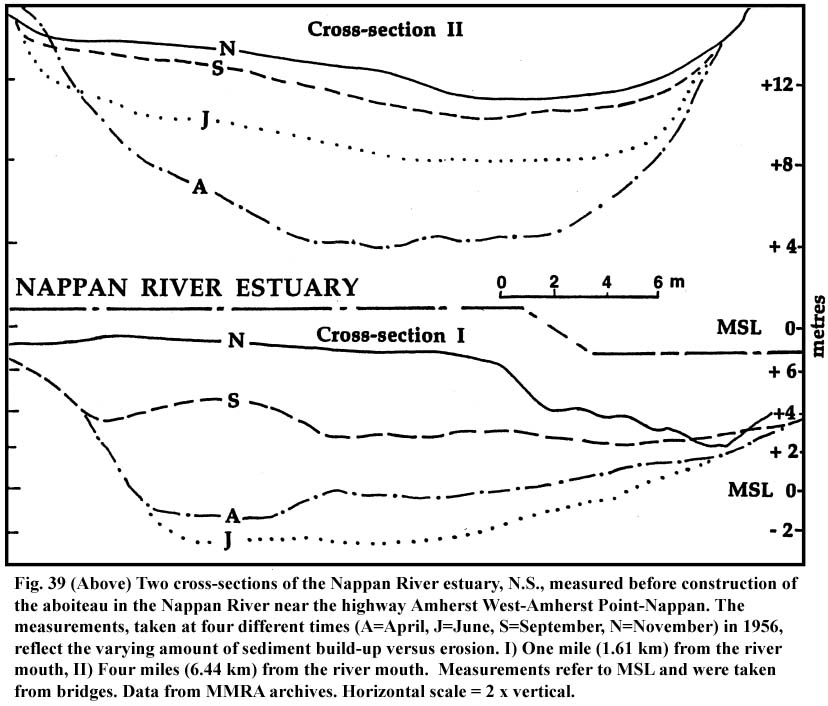
Display large image of Figure 39
196 Uplands, or freshwater bogs in the case of extensive salt marshes, form the landward limit of the high marsh. The latter situation can be explained by the fact that most of the sedimentation that occurs when sediment-charged tidal water floods the marsh, happens soon after it enters the marsh, forming a natural levee. Thus a pond is formed between the tidal estuary and uplands. With submergence of the landmass, the levee becomes higher, and the pond, which receives thinner layers of fine-grained material, becomes deeper and extended horizontally. At a late stage of development the far reaches of these ponds receive hardly any salt water, thus allowing freshwater vegetation a chance to develop.
7.3. THE REVERSING FALLS – A UNIQUE ESTUARINE FEATURE
197 The Reversing Falls at the mouth of the Saint John River, N.B. is a perfect example of what happens when an estuary of limited cross-sectional area must serve a tidal prism with a large surface area. It was on Jean Baptiste day, 24 June, 1604, that the first Europeans in the region, Pierre de Gua, the Sieur de Monts, a Huguenot merchant, and Samuel de Champlain, Royal Geographer, discovered the mouth of one of the largest rivers on the eastern seaboard of North America. These pioneers and others who came later described its mouth in their logbooks and reports. According to the Jesuit missionary Pierre Baird (1611), "The entrance to this river is very narrow and dangerous, for a ship has to pass between two rocks, where the current is tossed from one side to the other, flashing between them as an arrow. Upstream from the rocks is a frightful and horrible precipice, and if you do not pass it at the proper moment, and when the water is smoothly heaped up, of a hundred thousand barques not an atom would escape, but men and goods would all be lost." (Raymond 1910). Doubtless Baird was well aware of the Indian legend concerning the hazardous entrance to Saint John Harbour. Here the Indian cultural hero Glooscap is said to have created the Reversing Falls when he destroyed a large beaver dam built across the river's mouth. (The remains of Glooscap's beaver dam support a popular restaurant!) The natural feature responsible for the legend lies at the downstream end of a 4 km long, tortuous river section. At Indiantown, water surface levels can vary between 0.3 m above Geodetic Survey of Canada Datum (GD) during periods of small river discharges, to 5.2 m above GD during extremely large runoffs. Two kilometres downstream of Indiantown the river suddenly narrows to 215 m, and a sill occurs about 4.5 m below GD (see Fig. 40). Downstream of this sill the channel deepens to 45 m below GD and steep rocks conspire to form a gorge 106 m wide, with the bottom 40 m below High Tide level and a cross-sectional area of 2125 m 2. During Low Tide the river at the reversing Falls is only 78 m wide and the cross-sectional area reduced to a mere 1400 m 2 (Fig. 41).
Fig. 40 (Left) Index map to the Reversing Falls on the Saint John River, N.B. See Fig. 41 for view of cross-sections A1– A2, and B1– B2.
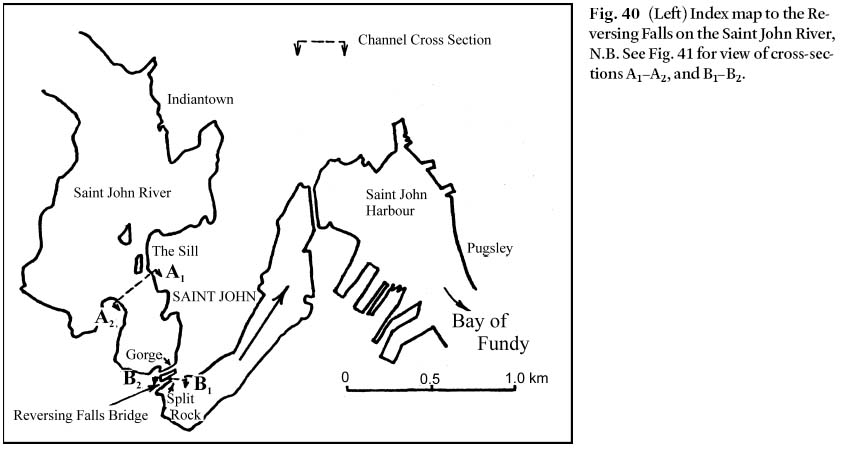
Display large image of Figure 40
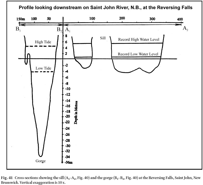
Display large image of Figure 41
198 The average freshwater discharge of the Saint John River is approximately 1100 ms -1. In spring, the melting snowpack in the watershed, combined with precipitation, can generate freshets of more than 10 000 m 3/s. The cross-sections over the sill and in the gorge are far too small to allow these storm discharges to pass at normal levels, which are little above MSL. Therefore at times the water has to rise over 5 m, even during low water, before such freshets can fully discharge into the sea. Even then, tides restrict the outflow twice a day during High Water. The average range of tide in Saint John Harbour is 6.7 m, reaching an elevation of 3.4 m + (above) GD. Large tides have a range of 9.1 m and reach 5 m + GD.
199 Upstream of the falls a system of drowned valleys (Grand Bay, Kennebecasis Bay, Long Reach and Belleisle Bay) provides drainage channels for the river and some of its tributaries. They have a combined surface area of 200 km 2 at the present sea level, and 250 km 2 at flood levels about 5 m above GD. Due to sea-level rise this system has gradually been filling over the past several thousand years. The tide has a range of about 0.5 m, but in the section of river upstream from Evansdale it is reduced to 0.3 m, and half that again 10 km further upstream. Upstream of the Falls the tidal prism is approximately 0.09 km 3, and can be filled within 6.2 hours by an average flow of 4000 m 3s -1 with an average velocity of 5.5 ms -1 through the area of 730 km 2 over the sill, requiring a drop of 1.5 m (Hansen 1970). When the river is low and with only a small gradient in the water surface, backwater effects due to the tides are observed near Fredericton, New Brunswick's capital, 125 km upstream of the falls.
200 In Saint John Harbour the tide ranges from – 2.0 m to +2.0 m with respect to MSL during small tides and from – 4.5 m to +4.5 m during large tides. Upstream of the falls the range is at most between 0.0 m and 0.6 m above MSL. This means that at High Water in the Harbour, the water will flow through the gorge and over the sill in a landward direction, dropping 1.75 m to 4.2 m depending on the strength of the tide. But at Low Water in the Harbour, the water will flow seaward dropping over a short distance 2.3 m to 4.8 m. Tidal water, augmented by the river discharge, gains a considerable velocity when moving over the sill where the available wet cross-sectional area is smallest. Rapids result in this section as the water moves turbulently through the gorge into the Harbour.
201 Navigation under these conditions clearly poses problems. Since tidal current and river flow are always present, there is no appreciable slack water in the Reversing Falls section. The ideal time to navigate the section is as close as possible to the time of slack water as indicated in the tide tables. Slack water at the end of the inward current is 2.4 hours after the time of High Water predicted for Saint John. The tide has then dropped sufficiently to be close to the same level as it is in the river upstream of the falls. Another slack time occurs 3.8 hours after Low Water, when the tide has reached the river level. Although slack water lasts less than 10 minutes, the section can be navigated for half an hour before and after this slack. Variations in meteorological conditions can alter the time of slack water by up to about an hour. At times it is impossible for ships to move upstream. An example is during spring runoff when river levels upstream of the falls are so high that they are not even reached at High Water levels of the tide. Under these conditions a steady seaward current will persist throughout the whole tidal cycle.
202 Flooding of the several lakes upstream on the Saint John River has troubled settlers on the fertile freshwater delta since 1694. In April 1987 heavy flooding associated with an ice jam caused water levels to rise over 5 m. The basic problem was recognized as early as 1693 by Lamothe Cadillac who, while conceding that the Saint John is the most beautiful, most navigable, and the most favoured river of Acadia, was all for blowing up the rock on which the Reversing Falls restaurant is situated. Indeed, the idea has been revived on more than one occasion since. Fortunately there has been strong opposition. People perceive that such a project would change the Saint John River into a tidal river with unsightly mud flats and alternating currents of turbid water. The remedy for protecting the low-lying lands would be worse than the problem because the annual inundation with fresh water would be replaced with inundations of salt or brackish water at every set of high tides. Moreover the Harbour would be ruined because tidal currents would become much stronger than they are at present, increasing the navigational hazards. For these good reasons the Falls remain a unique estuarine feature of the Fundy landscape.
7.4. TIDAL POWER
203 Tidal energy, exploited in Europe over 900 years ago, is highly predictable and is harnessed in much the same way as hydropower; all that is needed is a barrage across a suitable estuary that allows the bay behind it to alternately empty and fill with the tides. The greatest amount of energy available from falling water, at least in theory, is obtained by dropping the largest amount possible over the greatest vertical distance (Daborn 1977).
204 The construction and operation of a tidal power plant is however much more complex than a hydro plant on a river. At a given site, the amount of energy available depends on the range of the tides and the area of the enclosed bay. Since the head can never exceed the tidal range, unless water is pumped from the sea into the reservoir using energy generated elsewhere, the capacity of the plant can only be increased by moving more water through the turbines. This water must move by tidal action, within the period of 6 hours or less, from the sea into a reservoir when the sea levels exceed the reservoir levels. This water must then be temporarily stored in the reservoir until the tide drops enough to create a head that will drive the turbines. The larger the reservoir, the more power the plant can extract from the water. In principle it would be best to build the barrage at a point in the estuary close to the sea. Most estuaries flare and deepen toward to sea, requiring the barrage to be more voluminous and therefore more expensive and challenging to build. No matter what the location the control of tidal waters through the channel, particularly during the late stages of construction of the barrage, is extremely difficult. High tides during this construction period force large amounts of water through the closure gap. Nevertheless, in order to make a tidal power plant energy effective, an estuary is needed where large tides prevail. To illustrate (Bray et al. 1982; Gordon 1984; Gordon and Dadswell 1984), large sections of estuaries in the Bay of Fundy fall dry at Low Water. When the tide rises, the surface area of the water gradually increases. In most cases the water surface area for a trapezoid is approximated as follows:


205 The energy in a body of tidal water can be compared to the energy in the pendulum of a grandfather clock. The weight, or bob of this instrument, with mass m, is suspended a distance L from a rigid support. If the system is at rest, the force of gravitation will keep the bob at its lowest position, exactly vertical, below the support. However when the bob is drawn aside a distance x, it has to be lifted the vertical distance y. The relationship between y, x, and L can be expressed as:

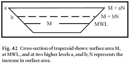
Display large image of Figure 42
206 The potential energy Ep is equal to 0.5 m · g · x 2/L, and the kinetic energy Ek can be given as 0.5 m (dx/dt) 2 , when x is small compared with L. The total energy is then the sum of Ep and Ek, and can be expressed as:

Table 16. Characteristic water surfaces, tidal prisms, potential energy, etc., of various sections of the Bay of Fundy
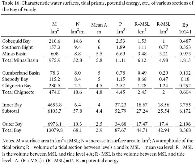
Display large image of Table 16
208 A body of tidal water can be likened to a pendulum lying on its side. At Mean Sea Level, its equilibrium position, the strongest currents occur and thus the maximum amount of kinetic energy (Godin 1990). The highest potential energy occurs when the surface is close to its High Water or Low Water positions. In order to reach its Low Water position, the water must be evacuated toward the sea by means of its current velocity. The water then has to move uphill, decelerate, and eventually come to a halt, thus limiting the volume that can be evacuated near the head of the estuary. Because this movement causes eddies and friction, the oscillating tidal movement can only be maintained when fresh supplies of energy are introduced into the system by the oceanic tides. Nor is all of the energy dissipated during each tide, otherwise the outgoing water would not have the energy to move uphill during the latter half of the ebb cycle and a noticeable imbalance between the High Water and Low Water amplitudes would result. There should also be a relatively large dissipation of energy otherwise the tide would not respond as fast as it does to the changing gravitational influences of the Moon and Sun.
209 The energy E1, of a layer of water with velocity v, density D, a surface area Sy km 2, dy metres thick, at elevation y, with the capacity of dropping a vertical distance h, and subjected to an atmospheric pressure p kPa, can be described as:

210 After the water has dropped the distance h, the energy changes in character. The potential energy Ep, represented by the factor D · g · h, is transformed into other energy forms, such as kinetic energy Ek, or heat energy Eh; it can also be extracted as electric energy Ee. Consequently the energy distribution E2 after the drop h, becomes:


211 Another interesting and important consideration concerns the value of N · y in (41) for Sy. When N · y is large relative to M, the potential for extraction of energy on the ebb flow becomes much more attractive than during the incoming flood flow because of the larger surface areas at higher levels of the reservoir. Double-effect extraction is less attractive (Larsen and Topinka 1984; Charlier 1982) because, although more time is available for extraction, the available head will be smaller, and very large sluiceways are needed in order to fill and void the reservoir of large volumes of water during shorter intervals.
212 Promoters of tidal power usually use the following simplified equations for calculating the potential energy extraction. Here it is assumed that the base level to which the water in a reservoir can fall is at elevation z, and that the total energy E e can be derived by the integration of the following equation:


213 Promoters may replace Y by the tidal range, and use twice the value, indicating a double-effect operation in which the reservoir is emptied simultaneously at Low Water, and filled again instantaneously at High Water. This yields a highly inflated value of the potential power extraction.
7.5. PROSPECTS FOR FUNDY TIDAL POWER
214 Greenberg (1987) has calculated the mean potential energy of the Minas Basin at 1.15 · 10 14 J per tide. For a smaller area (850 km 2, east of Cape Split), Godin (1990) estimated energy output at 2.657 · 10 14 14J. The theoretical potential energy for this area, calculated using (52), and Y as the local amplitude of the mean tide, is 1.8 · 10 14 J per tide. However, Charlier (1982) claims that a total annual energy of 169.5 billion kWh can be generated (this is equivalent to about 8.65 · 10 14 J per tide) with a double-effect unit.
215 A single-effect power station lets the water flow through the turbines in one direction only, generally from the basin into the sea, thus utilizing the greater basin storage at the higher levels. Since the amplitude of the tide can vary between 60 and 140%, its mean potential value can be even higher. As the output is proportional to the square of the amplitude, the importance of a large tidal range becomes obvious (see Table 16). Tidal range is even more crucial in areas where the water surface area increases significantly. In practice of course all this energy cannot be tapped. This would require the reservoir to be filled to high tide level, and then almost instantaneously released when the tide is out.
216 Experts on tidal power development estimate that only about 25 to 30% of theoretical capacity can be realized. For example, the French tidal power station on the Rance River has a basin with a surface area of 22 km 2 and a mean tidal amplitude of 4.25 m. The theoretical annual energy output should thus be 1567 GWh. However with an annual output of 544 GWh, the efficiency is close to 35% thanks to refined computer software, which optimizes plant operation, including pumping and double-effect power generation. A similar system is operated by the Russians in Kislaya Bay, near Murmansk. It has a 1.1 km 2 basin and a theoretical annual output of 6775 MWh of which only 2300 MWh is realized. The Russian and French tidal power stations operate with reservoirs used as holding ponds to create large heads, and turbines to extract the energy.
217 Alternate Fundy tidal power proposals call for placing paddle wheels or egg-beater-type propellers in the flowing water, without confining the water to either reservoir or restricted channel. One possible location is the Minas Channel, where current speeds can reach 7 to 8 knots. A current speed of 8 knots can be generated by a head of 0.86 m. Theoretically, by building a dam in the Minas Channel, a head of 10 m can be created. This is 11.5 times the head that the paddle wheel can be subjected to under the fastest currents. Nevertheless, in 1916 the president of Acadia University, together with two members of its engineering department and the head of its business academy, formed the Cape Split Development Company. During summer, a survey was made of the topo-graphical and hydrographical conditions between Cape Split and Squaw Cap Rock (just offshore from the Cape). The maximum tidal current was clocked at 11 mph (4.92– 5.66 m/sec). A model was constructed of a tidal power contraption consisting of pairs of endless chains linked to concave vanes and led over sprocket wheels that would drive pumps. The idea was that the pumps would continually top up two 250 000 m 3 storage tanks erected on the 100 m high Cape Split. Water would generate electric power utilizing machinery built in four open sluices and housed in the 120 m-wide gap between Cape Split and Squaw Cap Rock. Although shares were quickly issued, the company dissolved in 1929.
218 There were a few early success stories relating to tidal power worldwide. Records show that tide mills existed on both sides of the English Channel as far back as the 12th Century. Similar mills were also in operation along the coastline of eastern North America shortly after the first settlers arrived. Some of the mills served several purposes. In 1634, a cove and marshland north of Boston were dyked off. A three metre-wide sluice admitted tide water, which eventually powered two grist mills, a saw mill, and a chocolate mill. Most of these plants were abandoned when more convenient sources of energy became available.
219 A modest proposal for Fundy tidal power was advanced by K.E. Whitman in 1944 for a double-basin scheme using the Maccan River estuary as a head-water pond and the Hebert River estuary as the tail-water basin. Hicks (1965) identified seven possible sites between Cape Split and the mouth of the Bay of Fundy, and between Long Island, N.S., and Cutler, Maine. That same year it was seriously proposed to build a barrage through the 5 km-wide Minas Channel. The channel is 100 m deep at low water, and a suggested dam at this site would have a volume of over 75 million cubic metres! At that date, only the Fort Peck dam in the U.S.A. was more voluminous. To handle the volume of material needed in construction would require exclusive use for two years of loading facilities equivalent to all those available at the world's largest shipping centre, Rotterdam.
220 There have also been proposals based on the difference in tidal range on opposite sides of the Chignecto Isthmus. Tides in Cumberland Basin have an average range of 10 m, while 23 km away, in the Northumberland Strait near Baie Verte the average range is less than 5 m. Many people have had the mistaken idea that the Low Waters of these tides are at the same level as the Fundy tides, tides on both sides of the isthmus being measured from Chart Datum. The fact is that each tidal station has its own Chart Datum set at some particular elevation below Mean Sea Level. (Chart Datums are set at elevations so low that the tide at any given location will seldom if ever fall below it). Thus, and contrary to some proposals that have actually been advanced (see for example, Pogany 1958), the perennial economic problems of the Maritime Provinces can not be solved by simply digging a canal through the isthmus and installing a tidal power plant on it.
221 A more thoroughly researched report was prepared in 1945 for the Government of Canada (H.G. Acres and Co. 1946) concerning tidal power development in the Petitcodiac and Memramcook River estuaries. However this report, like that prepared by the Atlantic Tidal Power Programming Board (1969) for the Federal and Provincial governments, concluded that development could not be justified under the prevailing economic circumstances. A different conclusion was reached in the Bay of Fundy Tidal Power Review Board (1977). Out of 37 possible sites, the three most promising were in the Minas Basin, Cumberland Basin, and Shepody Bay. According to the report (which really focused on the results of market research), the largest, in the Minas Basin, would be capable of generating about 5000 MW; it was given preference over runner-up Cumberland Basin.
222 Many proposals have been advanced to try and tap the power of the Fundy tides (for details see Desplanque and Mossman 1998a). To date, however, only a modest experimental plant exists in the Bay of Fundy region. Installed in 1984 and located in the Annapolis River estuary, this small unit (20 MW) uses a "Straflo" combined turbine-generator to extract energy on an ebb tide, using a tidal range of 4.5 to 10.0 m. It may ultimately be the pilot for a vastly more ambitious undertaking to harness the great tidal ranges of the Minas Basin. In any event the construction of barrages in tidal waters is a formidable assignment. At La Rance, the French built the power units (total 250 MW) for the plant under dry conditions by placing cofferdams part way across the Rance estuary (Table 17). The placement of the cofferdams at La Rance succeeded, but not without a few tense moments. The relatively small power unit (800 kW) of the Russian plant was built into a floating caisson, 36 m long and 15.35 m high, which was then towed to the site and placed on a prepared bed. To smooth this bed the Russians sent some divers to the bottom equipped with hand rakes. It is extremely doubtful that such a procedure could be used in Fundy waters. A submerged tide gauge held down by pieces of railway track was placed in the upper portion of Cumberland Basin on 21
223 May, 1978, in 12 m of water. The current carried it away, and it was never relocated despite a thorough search.
224 Closing off parts of estuaries in the upper reaches of the Bay of Fundy would be a complicated undertaking, comparable but more difficult than the massive works carried out for the Deltaworks in The Netherlands. The latter are carried out through the cooperation of government personnel working together with contractors and a labour force experienced in this sort of work for many decades. The Deltaworks actually began with the construction of the enclosure dam and the first polder of the Zuiderzeeworks in 1927. Before that, the best scientific minds (among them H.A. Lorentz, Einstein's mentor) studied the implications of the closure of the Zuiderzee. The practical knowledge gathered during operations on both the Zuiderzee-and Deltaworks have established that undertakings of such magnitude require a sound logistical base in order to guarantee success. Planning a tidal power facility is not just a matter of placing a line on often outdated maps, and launching a public relations campaign. It involves plans that incorporate basic facilities such as sheltering harbours, and requires a sound infrastructure for constructing the facilities. Within the rigorous timetable ordained by the unforgiving tides, many new techniques would need to be developed and perfected.
225 "Fundy Tidal Power – Update ‘ 82" (Baker 1982) stated, among other conclusions, that: "Significant reductions in overall cost of a tidal power plant can be achieved by shortening the construction period and that should be one of the objectives of definitive design" (Baker 1982). In order to reach this objective it would be imperative that labour peace is guaranteed during the construction period. The "Update" also calls for the construction of 50 sluiceways and 64 turbine caissons, each 59 m long, 39 m wide and 46.25 m high, to be towed and placed on mattresses. This latter manoeuvre is an extremely delicate operation to be carried out during the periods of slack tide with split second precision, and in very close proximity of previously placed caissons. Any error of judgement will result in damaging collisions or time-consuming strandings of caissons. The construction and transportation of these 16-storey-high structures would require the ultimate of technical know-how. From the human perspective, these structures would be enormous, but in fact they are as delicate as oversized aquariums. They will have to be placed on platforms that will support the caissons evenly; otherwise internal stresses can play havoc with the structures and their contained expensive turbines or sluice gates. The successful construction and emplacement of such platforms would be a colossal engineering feat.
Table 17. Summary of tidal power generating capabilities of various sites
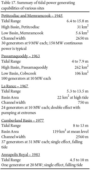
8. Ice Phenomena in a Bay of Fundy Estuary (TOP)
8.1. WINTER CONDITIONS: A SHORT CASE HISTORY
226 The transition from fall to winter in the Bay of Fundy is a time of stark contrasts. Huge amounts of ice can be formed in a few days of heavy frost. As we shall see, this can rapidly bring about dramatic change in the character of tidal estuaries in the Bay of Fundy (Jennings et al. 1993). On Wednesday, 10 December, 1980, the Sun was out, the wind was light, and the temperature hovered about freezing on the marshes bordering Cumberland basin (Fig. 43). No snow was on the ground and not a speck of ice in the estuary. A survey of ice conditions in the area, planned for the coming winter, was about to begin. The plan called for surveys on foot, on skis, and by helicopter throughout the period that ice would be present in the Bay. That day scientists from the Bedford Institute of Oceanography would be inspecting sites that the senior author had volunteered to visit during the winter.
Fig. 43 Index map of the northernmost portion of the Bay of Fundy shows various estuaries. Note too, the locations of causeways (C) across various rivers. LM marks the location of Lusby marsh. Inset shows New Brunswick (N.B.) and Nova Scotia (N.S.); location of Cornwallis River (CR), Burntcoat Head (BH), and the Shubenacadie River (SR).
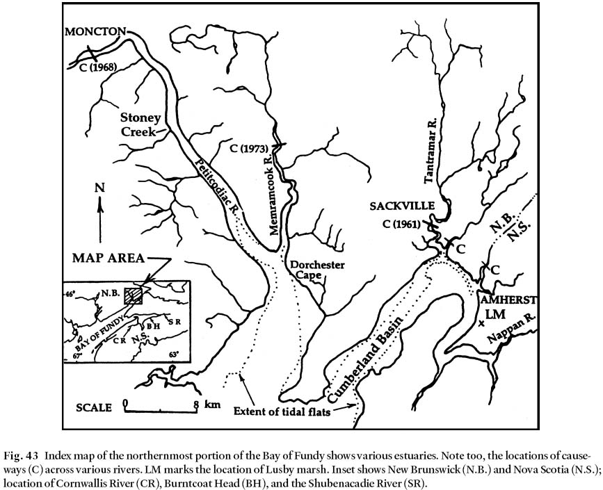
Display large image of Figure 43
227 By the following morning, as the temperature fell, the weather had changed significantly. On Saturday, 13 December, it was so cold and windy that it was dangerous to be out on the marsh alone. However on Sunday, 14 December, the Sun appeared again and conditions moderated. Five centimetres of snow covered the ground. In the morning, as the tide ebbed past Lusby marsh (LM on Fig. 43), one third of the ebb channel was covered with ice moving in the outside bend of the basin. Already formed were most types of ice common here in winter.
228 The drifting ice was mainly slush, or frazil ice, formed in open water areas termed "ice factories" (Knight and Dalrymple 1976), and made up of an unconsolidated mixture of needle-like ice crystals and sediment-laden water. There was also a good representation of pan ice, and cake ice. Pan ice, also present, is formed from accumulations of slush ice, frozen together in flat slabs up to 15 cm thick. Cake ice is considerably thicker, and probably forms as pan ice is jostled in fast-moving, ice-packed water. On its perimeter, cake ice picks up slush ice, creating an elevated ridge, or levee. The resulting basin-shaped central part can at least temporarily, hold silt-laden water. However the water usually seeps through the porous ridge leaving the silt behind. Collisions with other ice cakes evidently round the undersides of the cakes. Floating by too were a few scattered blocks of composite ice protruding 0.5 m and higher above the surrounding ice. On 14 December the only type of ice not yet in evidence was floe ice, normally formed where salinity and tidal energy are greatly reduced. Floe ice consists of frozen assemblages of all other types of floating ice, 50 to 100 m in diameter, that move restlessly with the tides, up and down the estuaries.
229 Following Desplanque and Bray (1986), the foreshore is here divided into three subzones (see also Fig. 44). The upper subzone is the vegetated high marsh that, in the upper reaches of the Bay of Fundy, is approximately 1.2 m below the highest levels that tides normally reach. Dominated by river-related processes, this subzone is not often covered with tidal water. During some winters, tides do not reach this level, in which case the high marsh escapes ice deposition (Dionne 1989). However, frozen crust, another major type of ice also present on 14 December, usually forms on the surface of the intertidal sediment. This "shorefast ice" results from the combined action of downward-freezing pore water, upward accretion of precipitation, run-off and, depending on the season, sea water (see also Desplanque and Mossman 1998b).
230 The landward limit of the high marsh is formed by dykes, uplands, or in the case of extensive salt marshes, freshwater bogs. On the seaward side a vertical scarp 1 m or more high separates high marsh from the middle subzone. In sheltered sections of the shoreline the upper portion of the middle sub-zone may be covered during the summer by Spartina alternifl ora (low marsh) and algae. Where rock is present seaweed may cling to it. Slippery mud, underlain by semi-consolidated material of similar grain size, covers the lower sections. The middle subzone has a relatively gentle gradient (approximately a 1 m drop in about 50 m), and its lower limit is also a scarp (Fig. 44) although not as high as the upper scarp. The lower subzone slopes toward the edge of the ebb channel, forming the thalweg (the median line of the channel) in Cumberland Basin.
Fig. 44 Different types of shorefast ice along tidal rivers and the upper edge of tidal flats. High marsh areas can be invaded by sea ice only during winters of extreme tides. Lower edge of shorefast ice bordering tidal flats may be floated at high tide. Slopes (vertical:horizontal), and generalized subzones (lower, middle and upper) as indicated. Modified after Desplanque and Bray (1986).
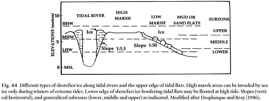
Display large image of Figure 44
231 On 14 December, 1980, the lower half of the middle zone was completely covered with cake and pan ice. Several centimetres thickness of silt had accumulated on some of the cake ice. On the upper half, a scattering of ice indicated the height of the tide during the preceding few days. The foot of the upper scarp had not been reached by the ice. In some places the lower subzone was covered with a crust of glazed ice beneath which water flowed toward the lower edge of the zone; in others, the ground was bare and unfrozen.
232 Several ice blocks stranded in the middle zone were constructed of 4 or 5 layers of ice of differing structure. Most layers were parallel, but some were oriented up to 45° relative to the others. The blocks, from 1 to 1.5 m high and 3 m square, contained much silt. However their buoyancy was very high because of the numerous air pockets. These sizeable blocks must have formed during the preceding three days because, as noted, ice was not present on 10 December.
233 During this three day period, the tides had not been large by Bay of Fundy standards; they ranged from a predicted 7.8 m + CD at Saint John on 10 December, to 7.3 m + CD on 14 and 15 December. However from this day on the tides became stronger, reaching a predicted height of 8.5 m + CD on 22 December. This semi-monthly inequality of 1.2 m at Saint John translates into an inequality of 2.0 m or more in Cumberland basin.
234 The weather remained cold. On 21 December it was unsafe to visit the site, but on 23 December we observed the effect of the increasing strength of the tides on the accumulation of shorefast ice forming along the shoreline in the zone between neap and spring High Waters. The middle subzone of the fore-shore was now filled with a thick layer of chocolate-coloured ice to 0.3 m below the level of the high marsh. It was impossible to reach the lower subzone because ice-covered crevasses between the cakes made the going extremely hazardous. Gradually the rising tide submerged the lower subzone and all types of floating ice covered the basin. Pan ice penetrated marsh creeks, becoming stranded on their banks.
235 Flat pan ice is commonly deposited on earlier-formed pan ice ferried in on weaker tides to freeze onto the banks. On higher parts of the foreshore stranded ice is left longer exposed to freezing air temperatures, and is more likely to become anchored to the banks (Sweet 1967). Commonly, ice may become bonded so strongly to a clay or silt substrate that it will not refloat when covered by a higher tide. In contrast, the connection between ice stranded on gravel or loose rock is rather more fragile. Sheet ice formed in the lower subzone of the foreshore moves up and down with the tides because the substrate cannot freeze during the shorter exposure to super-cooled air. This vertical movement of the sheet ice creates a bellows-like action between the ice and soft mud, promoting vigorous erosion.
8.2. THE PHENOMENON OF ICE WALLS
236 In the upper reaches of tidal estuaries, sea water can bring in ice that gradually builds up high vertical walls. Forced into the ever-narrowing sections of the estuary by a sort of ratchet movement, the ice is unable to exit. Initially, ice walls are rather porous and irregularly-shaped accumulations of ice. However, passing tides charged with floating ice cakes smooth off the rough edges, filling the pores and leaving a film of silt-laden water to freeze into a smooth surface layer of ice. Before long the trapezoidal cross-sections of tidal creeks, with side slopes of approximately 1:3.5, are transformed into rectangular channels of much smaller cross-sectional area (Gordon and Desplanque 1981). This in turn reduces the tidal prism and eventually also the flow rate of tide in the estuary (see Fig. 45).
Fig. 45 Diagram showing development of shorefast ice in forming an ice wall in a cross-section of a Fundy estuary delineated at day 1 (T0) by High Water associated with a neap tide, during periods of freezing temperatures, and at day 7 (T14) by High Water associated with a spring tide. After Desplanque and Bray (1986).
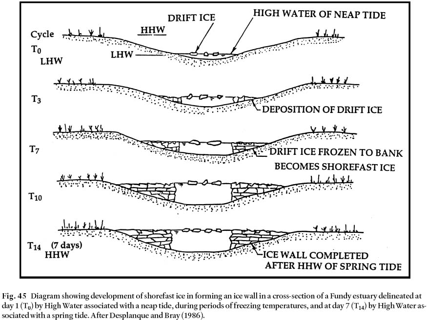
Display large image of Figure 45
237 During winter, ice walls 5 m high can build up in a week or less. Typically, ice forms a levee that is higher beside open water than toward the bank of a tidal creek (see Figs. 46, 47, and 48). These figures illustrate that impressive ice walls can form even in years of moderate tides. The foot of an ice wall tends to be slightly lower than the level reached by the lowest High Waters occurring during the frost period. Most of the ice becomes stranded shortly after High Water. Slack water intervals in tidal creeks are brief, to the point of non-existence. They occur after the water level has dropped following High Water. At High Water the water continues to move into the estuary on its own inertia. This process delays filling of the upper parts of the estuary with tidal water. Thus at High Water the ice is still moving in, to become stranded shortly afterward. Ice that is lifted onto the top of the banks or onto previously stranded ice will likewise be left high and dry when the ebb sets in. Before the next High Water the chances are good that this ice will become solidly frozen to the underlying base and will not be refloated. If it does manage to break loose, this will occur on the rising tide and stranding will occur at some point further into the estuary. The process sounds mundane perhaps, but in actual fact it is a most remarkable exercise in ice block gymnastics. The performance seems surreal because the delayed release of ice blocks from the substrate beneath the rising tidal waters causes them to be released by buoyancy, as if possessed of life.
Fig. 46 Memramcook River at College Bridge, N.B., spring 1959 (see Fig. 43), shortly before noon. Note how bridge piers influence movement of ice, incoming on the tide. A natural levee, formed by ice, is commonly higher near open channels than near the banks, a condition which can lead to flooding of the more inland shore ice. Note that this and following numbered photographs were taken for the Government of Canada (DREE) by Clifford Banks, and are used with permission; this is Photograph # 359-137.

Display large image of Figure 46

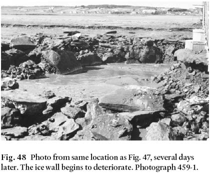
8.3. ASTRONOMICAL CYCLES AND ICE BUILD-UP
238 Ice build-up will be heavier during some winters than in others because of tidal conditions (see Fig. 49, Table 18). Peaks of perigean tides and spring tides coincide in cycles of 206 days. Two of these cycles last 412 days with the result that from year to year the especially strong tides occur 47 days later than in the previous year (412 – 365). During the first half of the 206-day cycle, the difference in height between neap tide and spring tide is decreasing, or below average, allowing a lesser ice wall build-up. Conversely, during the second half of the cycle, tides will gradually rise to higher levels during the week before the perigean tides. One of the key ingredients in heavy ice build-up is thus the timing of the greatest difference between neap tide levels and spring tide levels. This occurs one or two months before the perigean and spring tides combine to form the strongest tide of the cycle. Thus, when the latter half of the 206-day cycle occurs during the frost period between December and the end of March, one can expect the greatest build-up of ice walls. The formation of high ice walls in the Bay of Fundy was first recorded by Henry Y. Hind on or near 25 April, 1875 (Hind 1875). One hundred days earlier, the spring tide will have been at its minimum. Thus, the latter half of the 206-day cycle fell during the first period allowing ice to accumulate on the strand a month early, with accumulation probably peaking toward the end of April.
239 Naturally, the ice walls on either side of an estuary converge inland. Near the upper end of the estuary they will almost touch, leaving a strongly reduced channel in which freshwater runoff takes over the main role in channel-shaping. The drastic reduction in cross-sectional area can lead to flooding during a sudden winter thaw or spring break-up. The channel may then become choked with freshwater runoff, and/or ice. Certain rivers, such as the Salmon River near Truro, N.S., seem more prone than others to such flooding.
Fig. 49 Some tidal characteristics related to the ice regime in northeastern estuaries of the Bay of Fundy. Ranges and variation of tidal amplitude, Shepody Bay, showing the range over which particular types of ice occur.
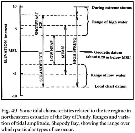
Display large image of Figure 49
Table 18. Summary characteristics of major constituents of tidal cycles in upper sections of the Bay of Fundy
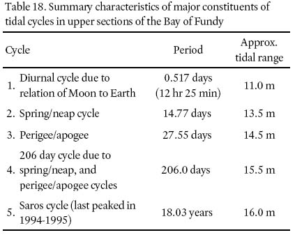
8.4. HAZARDS VERSUS BENEFITS OF ICE WALLS
240 The development of ice walls can contribute to disastrous problems in tidal waters. In 1965 a fertilizer plant was built at Dorchester Cape, N.B., near the confluence of the Memramcook and Petitcodiac River estuaries (see Fig. 43). In order to handle the bulk material to and from the plant, a wharf was constructed nearby. Because of the large local tides, a $2.5 million floating dock was constructed in the form of a 25 m × 90 m × 7 m concrete caisson connected to a wharf and concrete platform on shore by means of a bridge and connecting arms. At this location (see also Fig. 3) the average range of the tide is over 11 m, increased during large tides to more than 15 m. Since trucks had to move over the bridge the slope needed to be maintained within certain limits. Hence the distance between platform and caisson was substantial. Also, the tidal channel was dredged, allowing the caisson and ships tied to it to move freely up and down with the tide.
241 The facility, named the Port of Moncton, was officially opened on 24 November. Winter followed the departure of the first ship. An ice wall developed along the shoreline, and worse, between the platform and the caisson beneath the caisson arms. When this wall became sufficiently high and strong, it blocked the free movement of the connecting arm and bridge. The bridge lifted out of the water, the connectors buckled and broke, and the caisson drifted away, stranding on a nearby silt flat. The entire operation was subsequently shut down. Ironically, predicted and observed tides for November, 1965 were low, so that ice conditions might have been a lot worse!
242 What are the ecological implications of ice in the upper reaches of the Bay? At one time it was believed that ice moving from the high marsh during winter was the main agent responsible for transporting organic matter from the marsh into the Bay. However during most winters, ice is unable to move onto the high marsh. Thus the organic detritus of high marsh vegetation survives until spring only to disappear beneath fresh vegetation in the same manner as non-cut grasses on upland meadows, presumably by microbial decomposition.
243 Decaying high marsh vegetation is commonly deposited along the dykes in thick accumulations (Nova Scotia Department of Agriculture and Marketing 1987). Hydraulic conditions on the marsh are such that they inhibit most if not all seaward movement of organic debris; flow is too gradual at these shallow depths to accomplish transport.
244 On the low marsh, exposed vegetation is crushed and frozen into blocks of ice. Subsequently these blocks may be lifted by the spring tide, pulling the encased vegetation from the marsh. Removed to higher elevations they will remain stranded until the ice thaws, leaving the vegetation behind. In tidal rivers, ice walls begin to collapse by the end of March and most ice disappears except for shorefast ice that may persist until late April (see Figs. 50, 51). Stranding of large blocks of composite ice on the mud flats, acting in concert with the bellows action of sheet ice hinged to the shoreline, may cause the complete reworking of the soil under the sheet ice during the late winter and early spring. In late spring some tidal flats resemble plowed fields with great scars left by chunks of moving ice. Any form of life in this mudflat ecosystem survives only under a great deal of stress (Gordon et al. 1985). Macrofaunal diversity is very low. In addition to organic secretions of diatoms, most of the productive biomass derives from three species (Hicklin et al. 1980): a bivalve ( Macoma balthica), a polychaete ( Heteromastus fi liformis) and an amphipod ( Corophium volutator). The amphipod, so important to migrating bird life in the Bay, is widely distributed over the mudflats. Its survival in winter is doubtless predicated by its ability to burrow well beneath the zone of scour and erosion. Since ice scouring is most intense on the outer portions of mudflats, the role of shorefast ice may afford an important protection to these species in the inner several hundred metres of mudflats at the mouths of estuaries. Corophium volutator may also occur on exposed tidal flats with no ice.
Fig. 50 Tantramar River at the Middle Marsh Road, Sackville, N.B., 22 March, 1954. Here, the ice wall formed in January and had some ice cakes deposited on top of it during the high tides in February. Shorefast ice is starting to break up. The rough sides of the ice wall show that not much water is reaching it during High Water. Fundy tides were relatively low during 1954. Photograph #354-3.
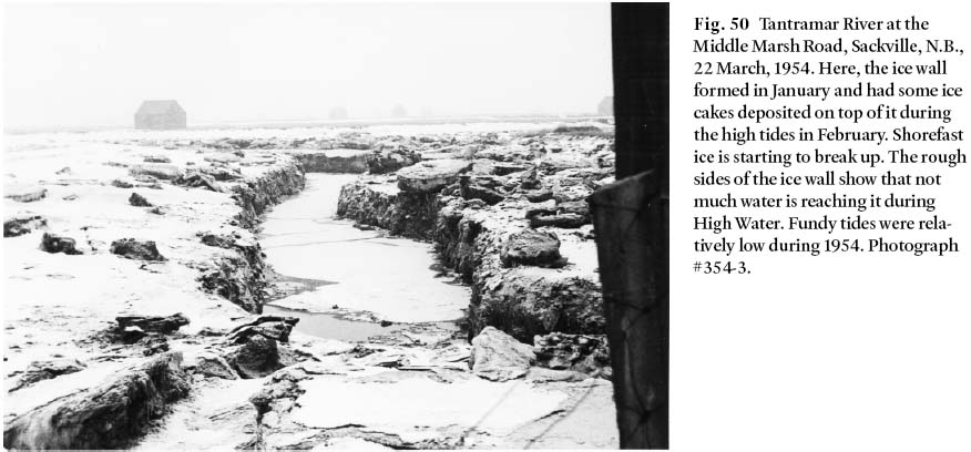
Display large image of Figure 50

Display large image of Figure 51
245 With approaching spring, flows of freshwater and tidal water progressively undercut the basal portion of ice walls and ice blocks. In places the ice is sculpted into dark-coloured, ephemeral toadstool-shaped formations charged with concentrations of estuarine mud as high as 18g per kg (i.e., 18 wt %) mud. By early April the thinner ice will have disappeared, but ice walls may persist until month's end (Fig. 52). At their base, huge accumulations of silt occur in sections sheltered from strong currents. It is remarkable that the ice fields are in the same locations where silt built up after construction of the Petitcodiac River causeway in 1968. Causeway construction promotes silt accumulation, with concomitant depth reduction of tidal rivers, and dire results for much aquatic life (Daborn and Dadswell 1988). With hindsight it can be seen that the river and its ice accumulations act like an enormous hydraulic sluice. Thus, whereas ice walls and associated phenomena may prove hazardous to man-made constructions they serve very important natural purposes. In the case of ice walls, their smoothness resists further narrowing of the channel, increases the net ebb and river flushing currents, maintains river depth, increases the surface slope seaward, forces the salinity intrusion seaward, and obstructs massive influx of ice from the estuary mouth.
Fig. 52 Petitcodiac River at Moncton, N.B. View southeast from Bore Park toward Dieppe, 11 March, 1959, shows extensive ice field in the river and the nearly vertical ice wall separating it from a secondary channel. Photograph #359-204.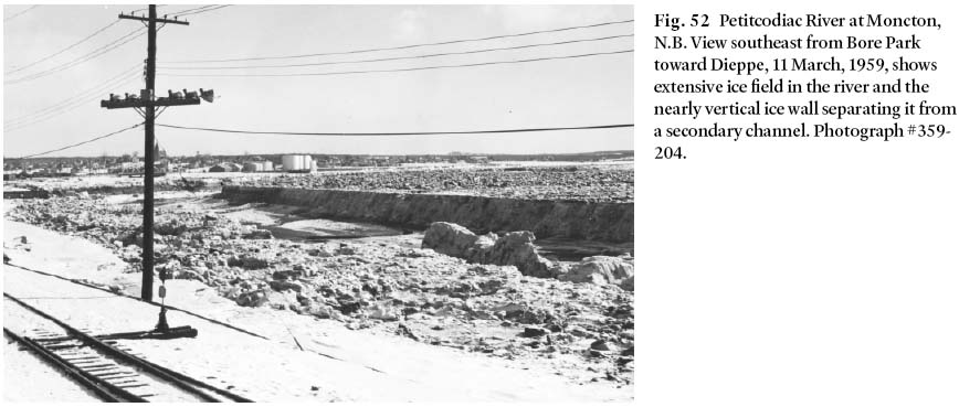
8.5. ICE-RELATED PROBLEMS IN ESTUARIES OF THE BAY OF FUNDY
246 There are many lessons to be learned from a consideration of winter conditions in a tidal regime as complex as that of the Bay of Fundy. Intertidal ice is an extremely active agent in diverse environmental processes, both physical and biological, in this macrotidal region.
247 From a strictly engineering perspective, the sequence of tides, temperatures, and wind velocities must be carefully evaluated in estuaries in northern regions subjected to a large tidal range. Floating structures attached to an estuary bank are at risk due to build-up of ice walls. So too, are bridges, where ice build-up increases the size of bridge piers, resulting in reduced cross-sectional area at the crossing (Figs. 53, 54). Construction designed to control flooding of marshlands must consider the downstream channel changes from trapezoidal to rectangular as ice factories swing into production. Shorefast ice can greatly inhibit the workings of one-way drainage devices, whether mechanical (flap gates) or electrical (gate slots), on hydraulic structures that are installed without due regard to winter conditions.
Fig. 53 Tantramar River downstreamof former Highway 2 Bridge, Sackville,N.B., 12 March, 1959. Note the coating of ice on bridge piers obstructing the flow of the tide. Some sheet ice has formed. Smaller ice blocks are stranded on top of larger ones. Photograph #359-203.
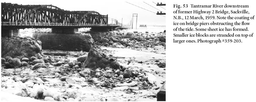
Display large image of Figure 53

Display large image of Figure 54
248 Concerning megaprojects like tidal power production, it is quite certain that a tidal power project would result in major changes in the dynamics and distribution of ice in an estuary. Reduction of tidal energy would promote water column stratification, which would extend the ice season. Sheet ice could expand near tidal rivers and by excluding extreme tides, the development of shorefast ice would be retarded. Not least, accumulation of drift ice at the barrage would need to be considered at the early design stage.
249 February is usually the time of heaviest ice build-up. Ice jams (dams) are most likely to occur in the upper part of an estuary during a period of low temperatures and spring tides. Conditions in the Bay of Fundy will be greatly exacerbated by strong, prevailing southerly to southeasterly winds that might coincide with a rapid thaw and heavy rains. Doubtless the most important factor affecting intertidal ice conditions in the Bay of Fundy is the unusually high tides. This results in several conditions not commonly encountered in other regions. Thick ice walls may be unique to Fundy estuaries due to the pronounced variation in the elevation of High Water during the spring/neap cycle, and the prolific High Water stranding of drift ice. Also unique, as we have seen, is the substantial variation in elevation of extreme (extraordinary) tides over longer periods than the spring/neap cycle. This factor affects the extent to which shorefast ice develops, and the degree to which the high marsh areas are influenced by sea ice. Hind (1875, p. 193) elegantly described the behaviour of ice in the lower zone of a Fundy estuary: "The appearance of an estuary in the Bay of Fundy at any time in midwinter presents some singular and striking phenomena, which may contribute to our knowledge of the manner in which different agents have assisted in excavating this extraordinary bay, and are now engaged in extending its domains in some directions and reducing it in others." At the time, his concern was with the potential impact of ice on the Baie Verte canal, proposed to link Cumberland Basin to the Northumberland Strait. Although this project was never completed, various large scale construction projects and a multitude of smaller scale coastal management and development schemes will continue to merit quality time applied to the task of understanding the dynamics and environmental effects of intertidal ice.
9. Sea-level Changes and Tidal Marshes (TOP)
9.1. POSTGLACIAL SEA-LEVEL RISE
250 In the Bay of Fundy region changes to shorelines are due primarily to tidally-driven processes of erosion, and to changing sea level through geologic time (Shaw et al. 1994; Stea et al. 1998). Because of its economic importance, the rise in sea level since initiation of the last deglaciation about 15 000 years ago, is subject to intensive study. In eastern North America generally, and in the Bay of Fundy in particular, abundant and diverse lines of evidence indicate that regional differences in sea level reflect postglacial isostatic compensation. A vast literature exists on this subject and debate continues concerning a link between a possible accelerated sea-level rise in response to a global warming (Peltier 1999). Here we focus on the nature of the dynamic interaction between land and sea as evidenced by erosion and the Holocene history of sea-level change in the Bay of Fundy.
251 Topographical maps give the heights of mountains as measured from mean sea level (MSL). The same maps are also quite definite in showing the location of shorelines. This assumes that MSL is permanent and known with a great degree of accuracy. Unfortunately MSL is a rather elusive concept. It certainly is not at a permanent elevation. The landmasses are ever so slowly bobbing up and down, and the oceans are not always filled with the same volume of water. Tectonic and isostatic processes contribute to an uneven sea-level rise along coastlines.
252 The future duration of the current interglacial is uncertain. During glacial maxima, large portions of the continents ringing the Arctic Ocean were covered with massive sheets of ice. The largest accumulation of ice during the last glacial advance occurred 20 000 to 18 000 years ago. In North America this last glacial is called the Wisconsin glaciation, and in Europe, the Weichselian (or Würm). At that time, so much water was locked up in ice that sea level globally was 100– 130 m below present MSL (Fig. 55). Across the Scotian Shelf, for example, this is indicated by a well-developed submarine terrace at a depth of 115– 120 m (Fader et al. 1977). In the Bay of Fundy, however, the terrace occurs at a depth of 37 m, a feature of fundamental importance to the distribution of surficial sediments in the Bay (Fader 1989).
253 Centered over Hudson Bay, the Laurentide ice sheet blanketed most of Canada and extended far south of the Great Lakes. It crossed the Bay of Fundy and Gulf of Maine, approaching the edge of the continental shelf (van de Plassche 1991). End moraines and glacial outwash peripheral to the ice sheet, and even some drumlins that formed beneath it, now form many of the banks and shoals along the Maritime and New England coastlines (Grant 1989). The rate at which the ice has retreated since the last deglaciation began is quite astonishing considering that the nearest remnant is now located on Baffin Island about 3000 km north of the Bay of Fundy. Most melting was over by about 5000 years ago (Lambeck et al. 1990). As discussed below, the rate of retreat was irregular rather than constant, due in part to eustatic change and spatially varying crustal motions, even during the last 1000 years or so (Shaw and Ceman 1999; Shaw et al. 2002). The current rate of rise of relative sea level is therefore not necessarily tied to an anthropogenic greenhouse effect. In any case, the sea was able to return in the western sections of the Bay of Fundy about 13 000 years ago.
254 The weight of an ice sheet is sufficient to depress the Earth's crust significantly. Compensating for this downward movement, the land and sea bottom in front of the Laurentide ice sheet was forced up into a bulge more than 100 m high and 60 km wide. With retreat of the ice, recovery takes place and the peripheral bulges gradually disappear. However, this process requires thousands of years, and in the Maritimes the recovery is still going on (Fig. 55). Thus, bulges that may have formed small islands off the Nova Scotian coast and a land bridge between southwestern Nova Scotia and New England, have gradually undergone submergence together with large portions of the mainland itself. For example, at the peak of glaciation, Georges Bank was 40 to 50 m above sea level. Yet 11 000 years ago conditions were such as allowed growth of salt marsh upon it (Stea et al. 1994; 1998). About 12 500 years ago the area of Portland, Maine was at least 49 m below sea level, and the sea covered nearly 23% of that State as far as Bingham, presently 100 km from the sea. Coastal areas along the Bay of Fundy also emerged as the ice retreated. Well defined former sea level stillstand indicators, such as raised beaches and nicks eroded in shore-facing cliffs, set the marine limits about 42 m above present MSL along Digby Neck and numerous other Bay of Fundy locations.
Fig. 55 Relatively short term, sea-level rise, from 15 000 years B.P. to the present. After Fairbridge (1987).
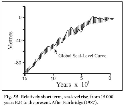
Display large image of Figure 55
255 From 11 000 to 5000 years ago, the land rebounded from the depressing effect of the ice (Grant 1989), and rose faster than sea level. Although over several intervals the rebounding effect reportedly slowed (Scott and Collins 1996; Stea et al. 1998), allowing reversals to occur, the tendency has been for the rate of sea-level rise to overtake that of the land. Consequently, submergence has occurred at a faster rate than that due solely to eustatic rise. Eustatic rise in sea level amounts to about 10 m in the past 7000 years. It is important to note that the inferred eustatic rate of sea-level rise of about 1.3 mm/yr is occurring globally, regardless of the vertical motion of any particular shoreline (Schneider 1997). This is the direct consequence of thermal expansion of ocean water combined with additional water mass derived from shrinking glaciers. Thermal expansion of the oceans is in itself is a very important factor, and although estimates in the literature range between 0.5 and 2 m/°C, the best estimates indicate that a 1°C rise in ocean temperature would result in a rise in MSL of about 60 cm.
256 Presently, sea level is rising all along the Atlantic coast of North America, but nowhere more rapidly than in Nova Scotia (Scott and Stea 2000; Fig. 56). This rise has been continuous for the last 7000 years at a rate of 20– 30 cm per century, accelerated between 5000 to 4000 yr BP when rates reached up to a metre per century (see Scott and Greenberg 1983). Tidal observations over the past 60 years confirm that the rate of rise remains about 3 mm/yr. For example, at Saint John, N.B., the measured rate is 3.6 mm/yr. At Halifax, sea level has risen 35 cm in the last 100 years; 20 cm is attributed to crustal subsidence, the balance is due to eustatic rise. Comparable rates occur along the coastline of the U.S.A. down to Florida. Along the northeast coast of Maine the rate exceeds 1 cm/yr. At places along the St Lawrence River estuary and the north shore of the Gulf of St Lawrence, the sea levels are not changing at present, although north of this line, for instance at Churchill, Manitoba, on Hudson Bay, land continues to rise relative to sea level (Hill et al. 1996).
Fig. 56 Mean annual sea-level change (1920 through 1990) determined from tidal gauge records at tidal stations in the Atlantic Provinces. Modified from Hill et al. (1996).

Display large image of Figure 56
257 While some areas were rebounding upward, other areas on the peripheral bulge were compensating for this movement and dropping in elevation (Scott et al. 1987). For example, at Lunenburg, N.S. sea level 7000 years ago was about 30 m lower than present, whereas peat that formed at the same time on what is now Georges Bank, can be dredged up from depths of 45 m.
258 During the last glacial maximum a glacier is believed to have occupied the Northeast Channel in the Gulf of Maine (see also section 4.3). The terminal moraine of this glacier may have served as a land bridge for the numerous species of plants that are native to southwestern Nova Scotia and southern New England but which are not found in the intervening coastal areas. Perhaps the Paleolithic people who settled in Nova Scotia 10 500 years ago used this land bridge to reach their hunting camps, the remains of one of which have been found at Debert, near Truro, N.S. (Grant 1975). Doubtless the existence of a land bridge restricted the free exchange of water between the Atlantic and the Gulf of Maine. The latter probably had a larger surface area than now because a large part of New England and the Maritimes was still covered with water. Today, with an average tide, about 300 km 3 of water flows in and out of the Gulf of Maine during a 12.4 hour period. If sea level was 30 m lower than today, the Northeast Channel in its present configuration would still have more than 75% of its cross-sectional area available for this flow. From a hydraulics point of view this restriction would have made little difference in the tidal characteristics of the area. However, if the channel was restricted by glacial material, and the surface area of the Gulf of Maine was much larger, tides of present strength could not possibly have been generated in the Gulf of Maine and the Bay of Fundy (Grant 1970).
9.2. MEMORIES OF THE MARSHES
259 Some very interesting features of tides and sea-level history in the Bay of Fundy, as discussed earlier (section 5.2), are substantiated in the geological record of tidal marshes. Marshes began to build up when tidal waters first covered coastal lands (Shaw et al. 1993). In the upper reaches of Cumberland Basin nearly 20 m of red clastic marine sediment have accumulated over the basal glacial till. Near Aulac, N.B., the marine sediments overlie a 6 m-thick layer of peat (Chalmers 1895). Given a compression ratio of about 3:1 or more for the vegetation to peat transition, the peat represents a formerly much thicker unit. The overlying silt will therefore also have been deposited at a higher elevation than it is now. Information from the drilling of wells has established that the lower limit of the clastic marine material is at a depth of 17– 18 m below the present land surface. This sets the lower limit of that material at about 12 m below present MSL. Thus constrained, the marshes could have begun to form 6000 to 7000 years ago when tidal ranges and currents became large enough to move material from eroding coastlines and deposit it in the upper reaches of the Bay.
260 During the summers of 1980 and 1981 students of the Free University of Amsterdam studied the development of marshes in Cumberland Basin (Dekker and Van Huissteden 1982). About 600 boreholes were made with an average depth of 6 m and a maximum of 15.1 m (Noordijk and Pronk 1981). One borehole, reaching 8.9 m below present MSL, was still in red marine sediment. The texture and structure of this material are similar to those of recently deposited clastic layers. No indication was found that the tidal regime at the time of deposition was any less vigorous than now. Marshes that are formed in areas with weaker tides have generally a much greater content of organic material. The same is true of tidal marshes less often inundated with salt water.
261 As we shall see (section 9.6), tidal marshes along the upper reaches of the Bay of Fundy are generally built up to a level about 1.2 m lower than the level reached by the highest astronomically-caused tides. At this level, relatively few tides are able to cover the marsh with silt-laden water. Each additional layer of silt progressively decreases the potential for more buildup. Combined with tidal cycles, marsh build-up is intimately related to the rate of coastal submergence. When sea-level rise is slow, marsh build-up is also slow, resulting in fewer inundations and prevalence of freshwater conditions on the marsh, especially in areas farthest removed from the coast and main creeks. Plant growth in basin areas on the marsh will resemble fresh marsh vegetation and will leave more organic peat-like material (Shaw and Ceman 1999).
262 Studies of soil genesis in the marshes reveals that there are 5 to 7 layers of organic (plant) material at particular stratigraphic levels throughout the marsh areas. This has been interpreted in terms of successive periods of increased and decreased rates of relative sea-level rise (Lammers and De Haan 1980). This phenomenon indicates intermittent temporary slowdowns in the process of submergence. Similar observations have been made in coastal areas of the northeastern United States, and of France, Belgium and The Netherlands along the North Sea. If, as suspected, intermittent submergence is a world-wide phenomenon, postglacial sea-level rise is a punctuated process, not necessarily linked to an anthropogenic greenhouse effect as suggested by Van de Plassche et al. (1998).
263 Temporary slowdowns of coastal submergence means that certain sections of the coast with exposed bedrock were exposed longer than others to wave action and consequent erosion. Tidal action during such periods will have remained the same except that the eroded material could not have been deposited on the marshes to the same extent as previously, but must have been choking tidal estuaries and creeks. This would lead to even less tidal water reaching the upper marsh areas. However, when coastal submergence was renewed, this material was readily available to be moved on the marsh, leading to an interval of renewed and vigorous marsh growth (Grant 1975). The geological record preserved in the tidal marshes is quite explicit in this respect (Figs. 57A, 57B).
264 Initial rise in postglacial sea level is signalled by the presence of fossil forests at several locations in the upper reaches of the Bay of Fundy. Typically, fossil tree stumps are rooted in glacial till at the base of the marine sequence; remnants of younger fossil forests also exist at higher levels. Among the intertwined network of roots, the peat-like consistency of the original forest floor is commonly well preserved. A good example occurs on the shore near low tide at Fort Beausejour on the Nova Scotia-New Brunswick border (see Fig. 3). The levels at which these stumps occur is approximately 1.2 m below present MSL. In 1983 more than 70 stumps were exposed, some with a diameter of over 1.5 m. Although most disappeared during winter of that year, fresh examples, including several blow-downs, have since been exposed. Pollen analysis of the peat indicates that the forest was a moist, rather patchy mixed-forest with hemlock, pine and red maple, which until its destruction by the rising waters was not disturbed by salt water (Grant 1985; 1989). The tree stumps have been radiocarbon dated at 3300– 3700 years BP. The maximum tidal range at Fort Beausejour is now about 15.6 m. Allowing 1.2 m for extraordinary storm tides, the stumps are approximately 10 m below the reach of a storm tide. This is compatible with a rate of submergence of about 3 mm/yr.
265 Although the section at Fort Beausejour is slumped, the relative sea-level curve obtained is reportedly comparable to those documented from several other locations around the Bay of Fundy (Scott and Greenberg 1983, p. 1556; see Fig. 57B). Most show a distinct break in the rate of sea-level rise at about 2500 BP.
Fig. 57 Sea-level change as evidenced in tidal deposits exposed at low tide on the shore at Fort Beausejour, N.B., at the head of the Cumberland Basin, in the Bay of Fundy. A) Section showing stumps and logs of buried forest at the base of the ca. 4000 yr succession covered by intertidal salt-marsh muds and peats. After Grant (1975). B) Relative sea-level curve for this locality established independently by Scott and Greenberg (1983).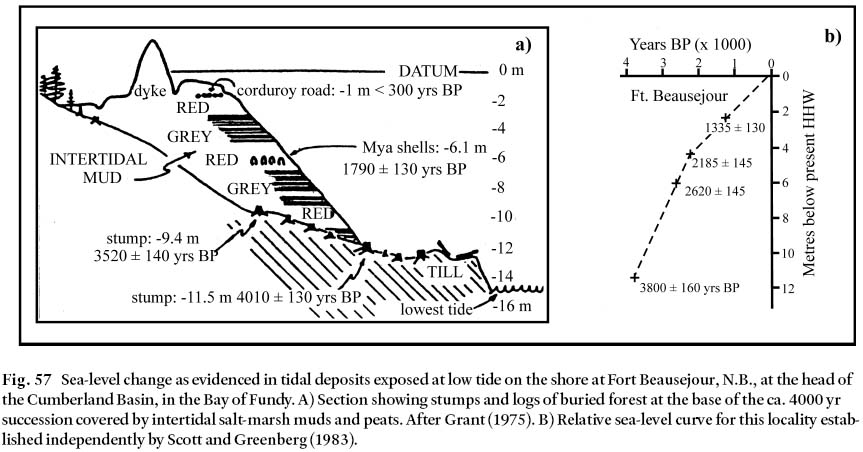
9.3. COASTAL EROSION
266 The more than 11 000 km coastline of the Maritime Provinces exceeds a quarter the circumference of the Earth. Of this, the coastline along the Bay of Fundy totals about 608 km in New Brunswick, and 805 km in Nova Scotia. Along much of this length, erosion-prone sandstones and conglomerates are exposed; along other stretches, "harder" rocks, like the basalt along much of the Nova Scotia coastline adjacent to North Mountain, offer stiffer resistance. Most resistant are massive igneous rocks, metamorphic gneiss and quartzite, and limestone. All are present in this geologically complex region. Erosion-resistant rocks form the headlands and capes, and each coastal section responds in its own way to the erosive powers of the tidal waters. Thus, one encounters 100 m-high cliffs, low bluffs, beaches, mud flats, tidal marshes and sand spits at various places along the coast, depending on local geological and hydrographic conditions. The difference in tidal ranges also leads to significant differences in the erosion of littoral materials.
267 In general, beach slope gradients depend upon the cohesion of the shore and bank materials and on local wave energy levels. Coastlines consisting of hard rock, such as the North Mountain basalt, are not easily broken down by action of wave and weather. However where bedrock consists of relatively friable material such as sandstone, the slope of the foreshore is formed of debris dislodged by wave action from banks and cliffs along the shore. Here the slope of the foreshore is uniform and gently dropping from 1:10 to 1:200, depending on local conditions.
268 Due to continuing submergence, a small section of back-shore, previously too high to have been exposed, becomes subject to wave action. Furthermore, the entire foreshore will be deepened so that wave energy will not be dissipated to the same extent in passing over it. Consequently wave attack on the shoreline becomes more vigorous. Equilibrium can be restored only if the foreshore is raised by debris removed from the freshly exposed backshore. Given the prevailing rate of coastal submergence and the evolution of the foreshore, the overall result is that the shoreline will have a tendency to retreat at a rate of 0.06 m to 0.8 m/yr depending on the slope of the foreshore and the resistance to erosion of shoreline materials. If the prevailing rate of submergence has been constant over the past 10 000 years, then sea level will have risen approximately 40 m since people first arrived on the shores of the Maritime Provinces, and 1.2 m since Père Pierre Baird described Saint John Harbour (see section 7.3).
269 The level of tidal waters lapping the shores of the Maritime Provinces is quite variable. Outside the Fundy region, tides are small, as in the western section of the Northumberland Strait (mean tidal range 0.6 m), or in the Bras d'Or Lakes, where the mean tidal range is 0.1 m. (The smallness of the range in the Bras d'Or Lakes can be brought home by the observation that changes in barometric pressure can cause differences in water levels of up to 0.3 m – Desplanque 1980; Petrie 1999.)
270 Wave energy is concentrated near the surface of the water. During high water the foreshore is covered by a significant depth of water and a far larger percentage of wave energy reaches the shoreline than when the tide is at low water. As noted earlier (see section 5.4.1), the zone of the shoreline near the water surface will be the most heavily subjected to wave action. Where water levels are rather constant, efforts at shore protection can be focussed in a limited zone. Conversely where macro-tides prevail, the problem of protection is complicated, and never more so than during perigean spring tides (Wood 1976).
9.4. COASTAL DEFENCE
271 In the Bay of Fundy tidal range in absolute figures is high. In the Minas Basin, tides have a mean range of 12 m and vary between 7 m and 16 m. Thus the zone in which the water surface meets the shoreline nearly 30% of the time varies between 2.8 m and 3.5 m above MSL during small tides and between 6.4 m and 8.0 m during large tides (Figs. 25, 26 and 27). This condition is clearly shown in terms of the amount of material eroded over a given tidal range. The exposed conglomeratic sedimentary rocks at Hopewell Cape, N.B., (see Fig. 29) provide an excellent example (Trenhaile et al. 1998; Desplanque and Mossman 2001a, 2001b). If any attempt is made to protect this sort of shoreline, then the zone requiring reinforcing needs to be at least 5 m high to have any effect. Attempts to protect shorelines are diverse: in many instances these prove to be expensive undertakings. Here we consider briefly one particular geological process all too often overlooked: the hydraulics of groundwater flow.
272 Due to density differences, fresh water can only move beneath the shoreline if it has an overpressure, because it needs to displace the heavier salt water. Should this overpressure dissipate because of friction and the pressures between salt and fresh waters become equal, then no transfer of water will take place. The plane where this situation exists is called the interface and its location is determined by the Ghyben-Herzberg ratio, which describes the static relationship of fresh ground-water and sea water in coastal areas (see Fig. 58).
Fig. 58 Idealized sketch shows the changing positions of the seawater/freshwater interface beneath a submergent nearshore island; h1 and h2 = respectively, the vertical distance between water table and the present MSL, and the vertical distance between the water table and the former MSL; 40h1, and 40h2 = respectively, the vertical distance between the present MSL and the present freshwater/seawater interface, and the vertical distance between the former MSL and the former freshwater/seawater interface.

Display large image of Figure 58
273 Fresh water prevails on the land side of the interface, salt water on the sea side. Because fresh water loses pressure gradually, the interface rises in a seaward direction and interacts with the sea floor at the elevation where the column of salt water exerts a little less pressure than that of the fresh water moving along the interface. This means that the excess groundwater has a smaller zone of exit into a saltwater body than into a freshwater body, and is much more concentrated, typically in wet areas near the shoreline. This concentrated outflow may cause quicksand and other soil/rock- weakening conditions near the shoreline where wave erosion is focussed (Figs. 59A, 59B). Furthermore, the fresh water exiting near the shoreline will expand upon freezing, promoting more rapid weathering conditions than might otherwise be the case. Also, since this groundwater is likely to be warmer than the air temperature during winter, many freeze-thaw cycles are possible during that season. In order to inhibit erosion of a particular section of shoreline, care needs to be taken to avoid local build-ups of freshwater pressure. Protective cover employed to this end should not be so permeable as to allow material to be easily dislodged. Incorporation of an artificial filter beneath the protective layer should be considered.
Fig. 59 Profiles show fresh groundwater encroaching on the foreshore. A) Water table is high, and fresh water moves onto the foreshore beneath the shoreline due to overpressure; soil/bedrock conditions are consequently weakened along the foreshore. B) Supposing that MSL is raised (or the water table is lowered by overpumping of the freshwater body), the interface between saltwater and fresh water moves shoreward. Saltwater incursion occurs, in part due to lack of freshwater overpressure. Arrows indicate hydraulic pressure flow lines; h1, h2, 40h1, 40h2, as in Fig. 58.
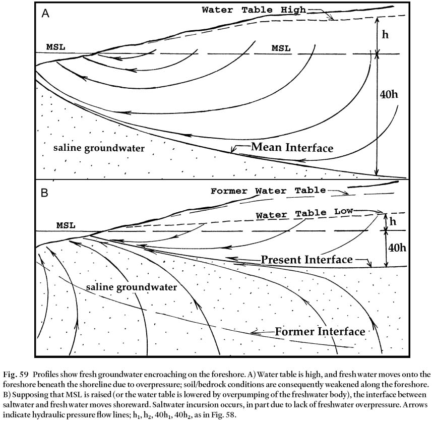
Display large image of Figure 59
274 Protection against coastal erosion is not only an expensive undertaking, but also involves high risks. The motto of a wise coastal engineer should read: "Be sure to put off to the future what you do not absolutely have to do tomorrow". The fight against coastal erosion is a struggle against strong and persistent forces in nature. Interaction of land and sea in the Bay of Fundy is a dynamic relationship. It is most obvious in recent cliff falls and in rapidly retreating bluffs as the sea advances inexorably and, at times of storm surge, disastrously. However, even on a decadal scale, continued sea-level rise is not always obvious upon cursory inspection. Measured in differences of several mm/yr, it is revealed in various sorts of tidal records, in bore hole data, and from radiometric and relative age data. At the head of the Bay of Fundy it takes the form of a startling paradox seen in the continued build-up of tidal marshes, as coastal submergence and erosion strive toward an equilibrium. Here, despite extensive dykelands, the marsh grows upward as sea level rises, yet recedes landward in the face of relentless erosion.
9.5. OVERVIEW OF MARSH TYPES
275 On a geologic timescale estuaries are ephemeral. The same is true for tidal marshes, because an extensive marsh occupies a natural estuary that has largely been infilled with sediment. A legacy of the ups and downs of the land surface in response to regional tectonics and climate, the system of tidal marshes extends around the Fundy shore, from Argyle and Chebogue south of Yarmouth, N.S., to the Musquash and Manawagonish marshes southeast of Saint John, N.B. (Fig. 60). They formed after the latest ice sheet retreated and mean sea level rose about 100 m to its present level, allowing tides to develop ranges and currents that could transport the sediment onto the marsh surfaces. Dyking was undertaken in the early 17th Century by the first French settlers, reclamation focusing along Cumberland Basin at the head of the Bay of Fundy. Johnson (1925) recognized three distinctly types of marshes along the eastern seaboard of North America:
- Coastal plain marsh. This type occurs south of New Jersey and is abundant from Virginia to Georgia. Related in structure to Fundy type marsh (below), it is developed in a regime of tides of much less amplitude. For this reason the marshes are flooded by each tide. This is because the marshes can only build up to a certain vertical elevation below the highest local tides and the difference in height is large relative to the variation in the magnitudes of the local tides. However the soils have a higher organic matter content and a different surface aspect than those of the Fundy marsh.
- New England marsh. Found from New Jersey to Maine, it differs from the Fundy marsh in that it is essentially a deposit of salt marsh peat with variable amounts of silt. The tides in this region too have a much smaller amplitude than those associated with the Fundy type. The Nova Scotia marshes in Yarmouth and Digby counties are of this type.
- Fundy type marsh. These marshes are built in a regime of tides with large amplitude and strong tidal currents. The high silt-carrying capacity of the Bay of Fundy currents cause marshes to build up with mineral matter, which is removed from the bottom, the banks, and the exposed shorelines of the Bay. Incoming tide water has a reddish colour and a silt content up to 2%.
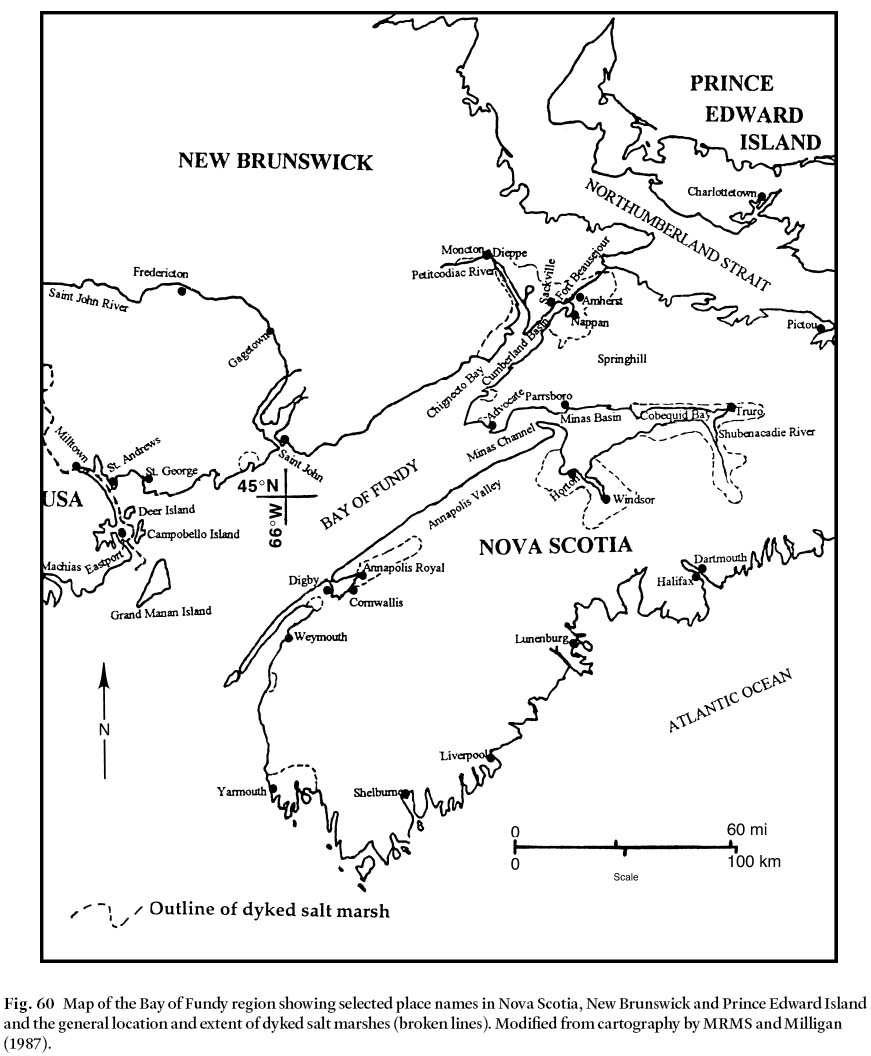
Display large image of Figure 60
276 We define a salt marsh as a low-lying flat area of vegetated marine soils that is periodically flooded by saltwater inundations, generally caused by tides, to such a degree that only plants adapted to saline conditions can exist. This definition excludes: a) unvegetated tidal mud, sand flats and gravel bars; b) sand and shingle beaches; c) dunes; d) dykelands, being former salt marshes, presently protected from tidal inundations by dykes and aboiteaux; e) freshwater marshes that exist between the larger salt marshes and the upland areas. The distance from the sea is so large that salt water cannot reach this zone within the limited time period available even during the highest tides.
277 Since a marsh creek needs a certain area of marsh to maintain itself against sedimentation, there will be margins of salt marsh free of creeks, along uplands and dykes, and between creeks.
9.6. TIDAL FLOODING AND MARSH GROWTH
278 The Fundy-type marsh, although built in a regime of tides with large amplitude and strong tidal currents, rarely experiences overflow. Tides that rise high enough to flood marshes in the upper reaches of the Bay, move larger volumes of water at higher velocities and greater eroding and sediment-carrying capacities. During large tides, High Water at the mouth of the Bay may extend 2 m higher than High Water during small tides. In the upper reaches, this difference can exceed 4.5 m. However, in the upper reaches of the Bay of Fundy the sea floor is too high to allow a Low Water. Therefore, it is better to employ the terms "large" and "small" tides rather than refer to tidal range, the difference between Low and High Water.
279 In general, tidal marshes in the Bay of Fundy area are built up to a level 1.2 m lower than the highest astronomical tides. Thus, only large tides can reach marsh levels and only very large tides are able to cover the marshes. For instance, on average, only 52 tides per year (standard deviation, SD, of the variation in tidal occurrences = 12) will be able to reach above the level of the remaining undyked tidal marshes around Cumberland Basin (see below). The number of tides that are able to cover the marsh to a depth of 0.5 m or more is 11 (SD = 5). These peak tides come in sets at monthly intervals, and a group of these sets appear at intervals of 7 months, 4.53 years and 18.03 years. Consequently, for long periods there will be no tidal flooding of the marshes. Thus Fundy tidal marshes can not be viewed as natural hatcheries or nursery areas for saltwater fish (Gordon et al. 1985). However when an overflow does occur, silt content of the water tends to be very high. Silt deposition on the marsh depends on the frequency of tidal flooding and the silt content of the tidal water. In the upper reaches of the Bay, the silt content is much greater than near the mouth of the Bay, although the frequency of tidal flooding is much less. Which factor is of greater consequence is open to debate. Sediment deposition upon the marsh causes a rise in elevation of the marsh in the same order as the rate of submergence of the region (Allen 1995).
280 In summer the soil can dry out, producing mudcracks up to 5 cm wide and 40 cm deep, a geological feature usually taken to signify prolonged aridity. The vegetation on such areas must be able to tolerate occasional flooding with silt-laden salt water, alternating with long dry spells (Gordon et al. 1985). Few species of plants are able to do this. Spartina alternifl ora, a pioneer in this environment, is able to withstand the effects of frequent flooding: however even this species has its limitations, and is able to grow in tidal creeks only to a level one metre below the marsh surface. The lower parts of the creek are bare of plant life. On the flat, high marsh another species, Spartina patens, is short and dense, promoting its requisite moist soil conditions over reasonably long intervals of time. Unfortunately neither species of Spartina contributes much fertility to the marsh, for they are short of plant nutrients such as calcium and phosphate. Nor is fertility enhanced by the silt-rich tidal marsh soil. These offer far less in terms of ion exchange capacity than, say, the calcium-rich clays of western Europe marshlands, or for that matter, New England marshlands (Desplanque 1952; 1985). As we shall see, intertidal flats of estuaries may vary seasonally, storing clay and silt during the summers and freeing them to winter waters (Amos 1995a, 1995b).
281 The apparent contradiction that marshes in areas with strong tides are less often covered with sea water than those where tidal amplitudes are low, is explained by reference to Table 19. Here, the height of High Water has been measured from Chart Datum, the average of the lowest predicted annual low water level over an 18.61 year period. Mean Sea Level (MSL) in the Maritimes has been rising relative to the landmass during the past several thousand years. Using all the hourly readings taken from 1927 to 1975, the variable distance between MSL and Chart Datum (CD) at Saint John, N.B., can be expressed as:

Table 19. Numbers of times per year that tides in Saint John, New Brunswick, reached to, or above, certain heights above Chart Datum (CD) and Mean Sea Level (MSL) during a 20-year interval (1947-1966)

Display large image of Table 19
282 Using the above relationship, as of 1 January, 1956, the value of Z0 was 4.270 m or 14.010 ft (MMRA. 1950– 1965). In Table 19, this value is used to estimate tidal amplitudes over a ten year interval. These data were used to calculate the S-shaped curve of Fig. 61, which shows the number of tides per year that will reach or exceed certain levels above Mean Water Level. According to the Canadian Tide and Current Tables, Mean Water Level (MWL) is defined as the height above Chart Datum of the mean of all hourly observations used for the tidal analysis at that particular place. At Saint John, N.B., there is most likely a changing difference in elevation between the MWL and the Geodetic Datum; hence MWL is used because it is linked to the local tidal movements.
283 Figure 61 is an example of what is known as a combination chart or nomograph, a type of chart widely used in engineering (Davis 1943). It does not have a horizontal axis (abscissa), employs a natural scale (rather than logarithmic), and displays the results of calculations which combine various functions (i.e., multiplication or division with addition or subtraction) based on observed tides at Saint John, N.B. The strength of the tides at several other stations in the region are represented in Fig. 61 by lines, the slopes of which are determined by the distance from the reference point (0 km) of Bar Harbor, Maine (see also Desplanque and Mossman 1998b).
284 From Bar Harbor, Maine, to the head of the Bay of Fundy the range of the dominant semidiurnal tides increases in magnitude exponentially at the rate of about 0.36% per kilometre. This rate is equivalent to 3.66% per 10 km, 43.2% per 100 km, etc. Given this 0.36% exponential increase in tidal range, when the high water level at Bar Harbor is 1 m above MSL, the level 196 km distant at Saint John can be calculated in the same manner as compound interest. The type of calculation is of course based on an exponential growth, and in this instance yields about 1 × 1.0036 196 = 2.02 m. Similarly, the ratio between Bar Harbor water levels and those 366 km distant at Burntcoat Head, N.S., is 1 × 1.0036 366 = 3.73 m.
285 Most salt marshes in the Bay of Fundy are raised to the level of the average tide, that is the MWL, in the 18-year cycle. Also, the number of high tides per year will vary considerably, depending on the phases of the three main tide-generating astronomical factors. As shown in Table 20, these coinciding peaks run in cycles of 0.53, 4.53 and 18.03 years.
Table 20. Analysis using simple multiples of astronomical cycles governing tides

Display large image of Table 20
286 Applied to variations in the levels of Bay of Fundy tides, the High Marsh Curve on Fig. 61 follows places where the local marsh level is assumed to be 1.2 m below the high water level during extreme high tides. It simply shows that the frequency of tidal flooding is much less in the upper reaches of the Bay of Fundy than in cases near its mouth. Drawn from a large data base, the S-curve in Fig. 61 shows the range in number of tides that can exceed a certain level. Taking the marsh level as an example, at Saint John it is approximately 3.5 m above MSL. The intersection with the S-curve shows that at Saint John the marsh will be flooded between 130 to 230 (C-B) times per year, depending upon when it happens during the 18 year cycle. At Bar Harbor, the number of annual floodings is between 660 and 700 (F-G), whereas the Cumberland marshes can expect only about 15 to 60 per year. (D-E).
287 Note also that the number of tides/year that will exceed a certain level at a given location is readily determined from Fig. 61. For example, with reference to Mean High Water (line X– W on Fig. 61), a minimum of 254 tides/year, or a mean of 354 tides/year, or a maximum of 433 tides/year (read off the ordinate), will exceed an elevation of 1.55 m (above MSL) at Bar Harbor, 3.10 m at Saint John, and 5.75 at Burntcoat Head (and 7.65 m at Truro). Although the data for Truro are not included, the last number illustrates the point that although the tide level at Truro exceeds that at Burntcoat Head, the tidal range is less at Truro because the floor of the estuary is higher and falls dry during ebb tides. The Shubenacadie River estuary, roughly midway between Truro and Burntcoat Head, illustrates the intermediate case: whereas the tide reaches its highest level about 9 km upstream on the Shubenacadie, MWL occurs at the river's mouth (see Fig. 36, curve 2, and contrast points L and B respectively).
Fig. 61 Combination chart showing the number of tidal floodings (read off the vertical axis) that can exceed a certain level on Bay of Fundy Marshes, based on observed tidal heights at Saint John, N.B. (1947 through 1966). The straight sloping lines from Bar Harbor, Saint John, Pecks Cove and Cumberland Basin high marshes give the corresponding tidal ranges. Mean High Water (MHW) and Extreme High Water (given in official Tide Tables for each station) are marked by the intersection of the sloping lines with WX and YZ, respectively. The Extreme High Water Level above Mean Sea Level (MSL) reached, for example at Burntcoat Head-Maccan, and read along YZ at K, is 8.7 m. The MHW level (A) at Saint John is about 3.1 m above MSL. The High Marsh Curve is an empirical auxiliary curve to determine the number of annual floodings of tidal marshes. Local marsh level is assumed to be 1.2 m below the high water level during extreme high tides. Where the High Marsh Curve crosses the sloping lines for the given tidal stations, vertical lines extended to intersect the S-shaped set of curves show the annual number of expected tidal floodings of out-to-sea marshes. Thus, for Bar Harbor, the number of floodings ranges between 660(F) and 700(G); for Saint John, between 130(B) and 230(C); for marshes along Cumberland Basin, the number of floodings ranges from only about 15(D) to 60(E).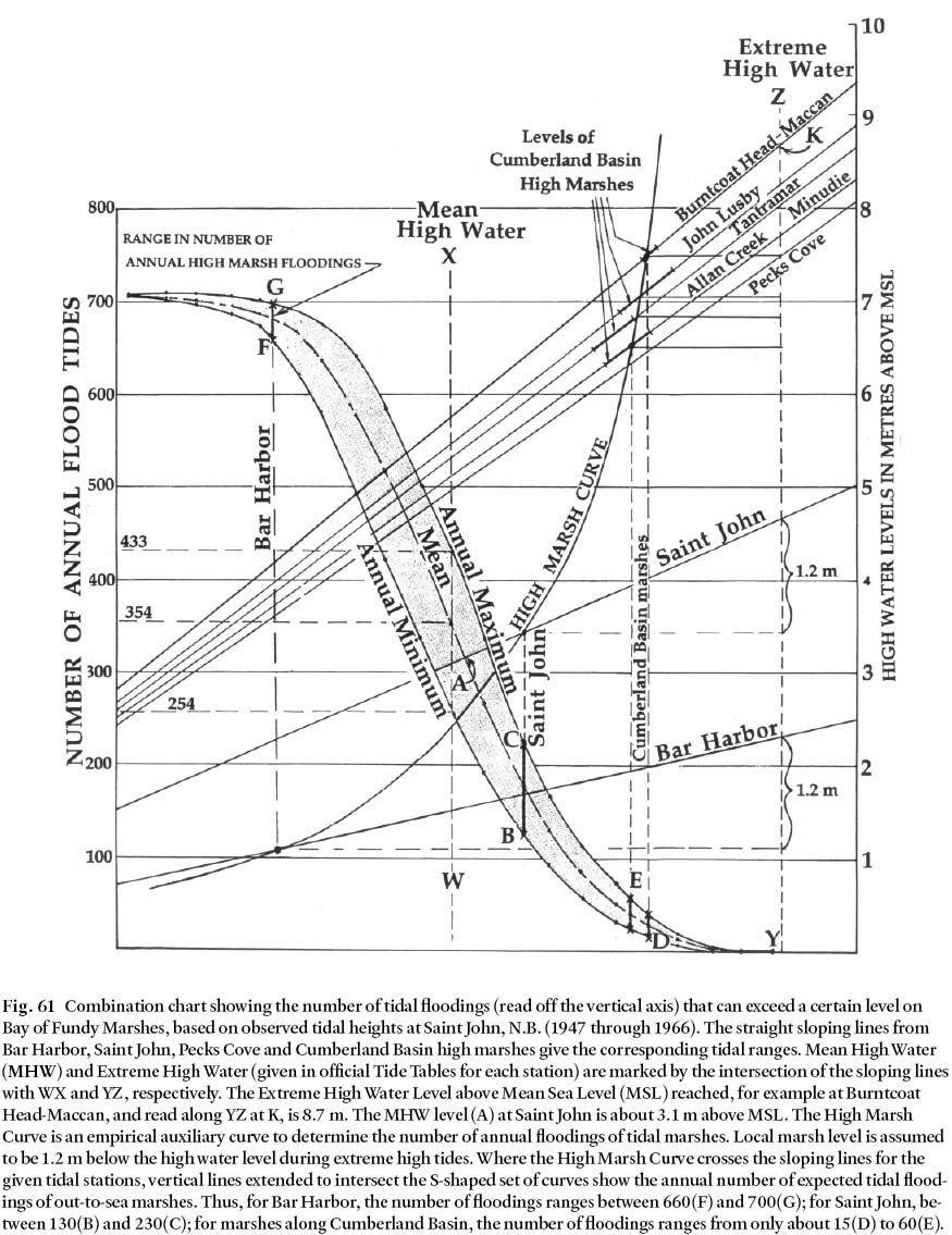
9.7. HISTORICAL DEVELOPMENT OF THE TIDAL MARSHES
288 In 1632, after about 25 years of exploration, colonization by Europeans of the lands surrounding the Bay of Fundy began in earnest. The settlers came from the Loire region of France, attracted by the coastal marshes. They were well acquainted with the techniques of dyking and draining in and around coastal marshes in their homeland as a result of activity by Dutch engineers invited to France in 1599 by King Henry IV. First to be reclaimed under this scheme were the Petit Poitou marsh along the Loire (1599– 1642) and the Petit Flandre marsh in the Saintonge district near Rochefort (1607– 1639) (Montbarbut 1985; Griffiths 1992). Early Acadian settlers applied the same techniques to tidal marshes in the New World. It was far easier to prepare this land than to clear thickly forested uplands (Fig. 62). At first the process proceeded peacefully. However, the struggle for political hegemony resulted in the forceful removal from the region in 1755 of approximately 10 000 settlers of French descent ("Acadians"). They were replaced by settlers from the British Isles and New England. The French had exploited to the limit the potential for dyking and draining the existing vegetated high salt marsh to form polders (van Veen 1939). Today 36 000 hectares of dykelands form a significant percentage of land suitable for agriculture in the Maritime Provinces of New Brunswick and Nova Scotia.
Fig. 62 Illustration shows the Acadians of Minas building of a dyke and an aboiteau near Grand Pré, Nova Scotia. Painting by Lewis Parker, in Dunn (1985, p. 11). Reproduced with permission.

Display large image of Figure 62
289 Elsewhere in the world are similar landscapes: the polder landscape of The Netherlands is often used as the prime example of this cultural environment. There, over 350 000 hect-ares of land have been reclaimed from the sea and another 1 300 000 hectares are protected against occasional storm tides. In Bangladesh 1 500 000 hectares of land are protected against tidal flooding, although 30– 40% of its land area (144 000 km 2) is flooded by river water during 4 to 6 months of the year. The technique of protecting such land is everywhere identical, with flood-prone areas protected against high sea levels by dykes. The dyked land is drained by means of gravity sluices or pumps. In the Bay of Fundy area, the tidal range is so high that during much of the day the sea level is much lower than the dyked land, no matter how strong the tide. This means that gravity drainage is possible almost all of the time. For smaller tracts of protected lands, sluices with clapper gates are used, while in larger projects, gates are operated electrically. Clapper gates allow fresh upland water to flow into the sea while blocking seawater from flowing inland over the marsh. Gated drainage sluices within the dyke are called aboiteaux. Although there are many versions of this term, the original word may have been abat-eau (protector against the water), similar to abat-vent (windshield), abat-jour (Sun shade) abat-son and abat-voix (sound boards). The version abateau remains in use in the Saintonge district of France.
290 Most of the dyked marshes in the Bay of Fundy occur at the head of Cumberland Basin, the central of three main arms of the Bay. Along the Basin, which has a surface area of 118 km 2, 147 km 2 of dykelands have been created. The Tantramar marshes east of Sackville, N.B., along the estuaries of the Tantramar and Aulac Rivers, form the largest block at (72 km 2), according to Griffiths (1992) "… the largest salt-marsh lands in the world…" (see Fig. 61).
291 The surface of most of the dyked marshes is 2 m or more below the highest level reached by the tides, while the salt marshes have an average elevation of 1.2 m below that level. Dyke elevation is of course partly attributable to the geologically recent submergence of the landmass relative to sea level in the Maritimes. Another important factor is the length of time that the dykelands have been deprived of additional sediment. For example near Amherst, N.S., dykes protecting the John Lusby marsh were breached during storms in late 1949 and early 1950. The damage was so extensive that no efforts were made to reclaim the land. The following tides built the marsh up a metre or more, burying fence posts in the process, the tops of which are now barely visible above the ground. Another important variable is the rate of erosion. Thus, although tides are higher in the Minas Basin, the coastline along Chignecto Bay is more easily eroded, and this factor may favour the greater abundance of marshes around Cumberland Basin.
292 The early French settlers, who were mainly subsistence farmers, used the dykelands for a variety of grain, oilseed and fibre crops, shifting later to beef production. The dykelands became the producers of the hay required to feed their livestock during the long winters. Centuries later, when means of transportation were improved and large population centres had developed along the eastern seaboard of North America, the excess hay was exported as fuel for the horse-drawn forms of city transportation. This lucrative enterprise stimulated the urge to increase the acreage of productive land. Most of the sediment carried onto the marsh is deposited in natural levees along the coastline and the tidal creeks leaving the more inland areas with much less sediment cover. As a result, the marsh surface slopes landward towards the edge of the upland where, in saucer-like basins and low-lying areas distant from the coast, freshwater bogs are common. At these sites, bogs with cat-tails and sphagnum vegetation are developed in a zone between the marsh and upland and, in some cases, even in the centre of a marsh. An example of the latter situation is the so-called Sunken Island Bog on the Tantramar marsh near Sackville, N.B. Underlain by marine clays, the bog is a prime example of a floating sphagnum bog surrounded by a fringe of vegetation, characteristic of wet conditions.
293 It may be no coincidence that after an article on "warping" or "tiding" was published in the British Farmer's Calendar of 1804 promoting the build-up of lands by tidal inundations in Lincolnshire and Yorkshire, a similar project was undertaken in the Tantramar region of New Brunswick. History records that many settlers from Yorkshire came to the Sackville area. Canals were dug between the Tantramar River and several nearby lakes, in the process transforming hundreds of hectares of freshwater peat bog into profitable grasslands.
294 At the mouth of the Tantramar River, tides have a maximum range of 14.5 m. As an employee of the Maritime Marshland Rehabilitation Administration (MMRA) in July 1952, the senior author made, with the aid of explosives, a 500 m long ditch from the Tantramar River to Long Lake, 22.5 km from the mouth of the river. Within about three years most of this 7.5 hectare lake was completely filled with silt for new farmland, and no longer appears on Topographical maps. The sets of very high tides in 1953 and 1954 contributed greatly to this last "tiding" carried out in the Bay of Fundy area.
9.8. REHABILITATION AND RECLAMATION
295 Through vigorous efforts, the early French settlers proved the feasibility of dykeland development and utilization. Many remnants of old Acadian dykes exist on sections of marsh that have since been allowed to revert back to salt marsh. It appears that these settlers built their dykes at the very edge of the salt marsh, leaving only a very narrow safety margin for waves to dissipate most of their energy during High Water (Baird 1954). In addition to earth, the settlers also used pole and plank facing. This same method had been used centuries ago in Europe to protect the face of dykes, but was abandoned after shipworm ( Teredo navalis) invaded the waters of northwestern Europe in the first half of the 18 th Century. The teredo consumed all the wooden parts of dykes and sluices and generally promoted wholesale rotting of poles and planking. Weaknesses thus created became foci for wave action, which continued the degradation until eventually holes developed in the dykes; the process is similar to that which results in sea caves and blow holes. Fortunately, teredo is not found in the Bay of Fundy, although it is present elsewhere along the North American coastline. Only a limited number of mollusc species are able to thrive in the upper region of the Bay of Fundy, the common periwinkle ( Littorina litorea L.) being a recent newcomer. The fact that plank facing is still used in Fundy dykes attracted the German geographer Carl Schott to the area in 1952 to study the application of this ancient form of dyke protection. His work (Schott 1955) remains the best comprehensive report on the Bay of Fundy marshes.
296 After World War II economic studies indicated that rehabilitation of deteriorated dykes and aboiteaux would be beneficial. Accordingly, the Federal Government financed and carried out the building or rehabilitation of 400 km of dykes and new sluices, while provincial governments and landowners agreed to share the cost of associated drainage facilities. Several former dykelands were in such a state that no rehabilitation was attempted. Of these lands, a few have been acquired by the Canadian Wildlife Service to serve as National Wildlife areas, some of which are important stopover and feeding areas for migrating waterfowl. Low-lying sections of the dykelands, especially those fringing the uplands, were dyked off internally and transformed into waterfowl habitat (work that is financed and carried out by that uniquely North American organization, "Ducks Unlimited"). Some tracts of dykeland are small parcels of land sandwiched between the upland and meandering tidal estuaries. The required height of the dykes is only about 1.5 to 2.0 m above the original marsh level.
297 Present-day dyke construction is carried out using bulldozers and draglines. Topsoil is first removed from the projected dyke site and stockpiled for later re-installation. The bulk of the dyke material is taken from the drainage ditch running inside and parallel to the dyke. Any necessary additional material is taken from borrow pits outside the dyke. The outside face on exposed sections of dyke is covered with quarried rock trucked in during the winter when the dykes are able to withstand heavy traffic. These rocks dissipate wave energy generated during High Water.
298 The dimensions of the aboiteaux or discharge sluices are determined by a number of equations that take into account potential storm runoff from the watershed to be discharged through the sluice, the ranges of the local tides, the elevation of the dykeland, and the sluice invert elevation allowed by the receiving tidal channel. For sluices built in larger creeks and estuaries the available storage volume of basins upstream of the sluices is taken into account, as well as the probable hydro-graphs of the storm runoffs.
299 The large tidal ranges in the Bay of Fundy permit exclusive use of gravity drainage. Pumped drainage is uneconomical and would only be required for short periods during High Water should tide water exceed the water levels upstream of the sluice, and only then if the storage volume was insufficient to hold the watershed runoff during that period. Such occasions would be so rare that the large capacity pumps would hardly ever be used.
300 Some 435 small aboiteaux were built by the Maritime Marshland Rehabilitation Administration in the 1950s and 1960s. Dimensions ranged from 0.3 × 0.3 m boxes to multiples of 1.2 × 1.5 m boxes, set side by side and made from chemically treated lumber. More recently, sluices have been built with asphalt-coated corrugated steel pipe. The flapgates are made of bronze or steel and hung by horizontal hinges or steel chains. The latter method appears superior for it allows debris to pass through the sluices with less damage to the gates.
301 To eliminate the need to rehabilitate tens of kilometres of dykes and numerous small aboiteaux, six large tidal sluices were built in larger tidal estuaries (those of the Annapolis, Avon, Memramcook, Petitcodiac, Shepody and Tantramar rivers). The largest of these structures are the five 8.8 × 8.8 m sluices (with inverts at 1.5 m below MSL) set in the Petitcodiac River estuary near Moncton, N.B. Two slightly smaller sluices in the Annapolis River estuary were converted in 1982 into an experimental tidal power station (see section 7.5). The large tidal sluices are steel-reinforced concrete structures with flared entrances and are equipped with electrically hoisted gates which can, if necessary, be operated manually. These gates can also be electrically heated for use during periods of heavy frost. In the larger estuaries the sluices were not able to pass enough water during the time of dam construction. Therefore auxiliary sluices were built to keep tidal currents in the closure gap at manageable speeds. Later on these sluices were buried within the dam itself. These dams also serve as causeways for highway and rail traffic, shortening the connecting links among the provinces to a significant degree.
302 The operation and management of dykelands are carried out under the direction of "marsh bodies", elected by landowners and assisted by officers from the provincial departments of agriculture. There are 86 such "marsh bodies" in Nova Scotia and 39 in New Brunswick.
303 The reclamation of Fundy tidal marshes has been regarded by some people as ecologically disastrous in light of recently publicized figures of salt marsh production. For example, in semi-tropical Georgia, Spartina alterniflora has been measured at 2883 gm -2/yr, a figure greatly exceeding that of other forms of natural vegetation or agriculture (see Pomeroy and Weigert 1981). In Virginia, the measured rate of production is 1143 grams, in Rhode Island 668 grams, and on high marshes around Cumberland Basin a mere 400 gm -2/yr. Factors responsible for the relatively low production of salt marsh vegetation in Cumberland Basin include: the shortness of the growing season, nutrient limitation, inundation characteristics, sediment aeration and, last but not least, tidal stress.
304 Unfortunately, the Georgia figures are most often used in ecological arguments naming the Bay of Fundy a disaster area. Simply put, Fundy tidal marshes can remain dry for months on end and thus cannot be construed as hatcheries or nursery areas for saltwater fish. The dyking of the high marsh in the upper reaches of the Bay will not have had the same biological impact as results from utilization of marshes in more southern latitudes, or in regions with smaller tides. Nor is there much basis for stating that reclamation of the salt marshes has been detrimental to the region's bird population. When the French settlers arrived in the upper reaches of the Bay, they called the area "Tintamarre" because of the birdcalls that filled the air. The present name of the Tantramar marshes derives from this word, which means din, racket, or noise. With this explanation comes the idea that the original undyked salt marshes had a rich birdlife. It is interesting to examine this proposition.
305 In The Netherlands, until recently, every hectare of reclaimed or unreclaimed marshland seemed to have its own resident couple of lapwings, godwits, and skylarks, and every acre of water its pair of mallards. This was the case despite the dense human population and intense agricultural use of the polderland. More intense agricultural practices and use of pesticides have recently changed this picture drastically. In contrast, Maritime marshes are almost devoid of birdlife, especially the out-to-sea marshlands. The French may possibly have named the marshes "Tintamarre" during the spring migration period when the marshes are staging areas for geese and ducks, or during the late summer period when hundreds of thousands of waders congregate at selected areas.
306 Overall, the Fundy marshes have very little bird life. Indeed, the salt marshes could never have provided suitable nesting habitats for birds because there is a total lack of trees. Furthermore, the infrequent monthly flooding of the marsh with salt water, which occurs in sets that arrive about 47 days later from year to year, makes the marshes unsuited for ground breeders. Since these floodings are more intense every 4 to 5 years, it seems improbable that bird species could have become used to monthly floods and incorporated them into their genetic programs. This leaves only breeding areas for birds like the raucous redwing blackbirds that can multiply among the cat-tails in transition areas between the salt and freshwater marshes. This may well have been the "tintamarre" that so impressed the French settlers.
307 The dyking of marshes has had another, less remarked upon effect (Teal and Teal 1969). Before dyke construction, tidal marshes acted as sinks for excess suspended sediment in the system. Following dyke construction, this suspended material may have resulted in changes to the habitats not only of plankton, but also of fish like shad and gaspereaux. Historical records show that in 1837, vessels from 50 to 150 tons were able to sail almost daily up Cobequid Bay and the Salmon River to receive and discharge cargo near the now defunct Board Landing Bridge near Truro (see Fig. 60). After 1867, however, siltation of the river prevented further shipping access. Similarly in England by about 1888 all the harbours on the southeast coast of England were silted up due to dyking of marshes, requiring a vast expenditure for constant dredging to keep harbours operational.
308 Very little use is being made of salt marshes for socio-economic purposes unless the terrain is transformed to dykeland. Dykelands provide pasture, especially for sheep, and a source of "wild" hay. Some plants such as Salicornia and Plantago were eaten as a vegetable on a minor scale (Trueman 1896). The marsh is generally inaccessible and unattractive to conventional recreation seekers. Fundy salt marshes are cold in winter, wet in the spring, mosquito ridden and covered with nearly impassable vegetation during the summer and early fall, and muddy throughout the year. In fact, smells emanating from marshes are usually so obnoxious that they have a serious effect on the recreational usefulness of adjoining shore properties. The only "recreational use" of salt marshes is the realization of their importance within ecosystems.
309 Today, although an estimated 90% of the original salt marshes at the head of the Bay of Fundy has been reclaimed by dyking, much of the rest remains idle. The once lucrative hay market has disappeared. Few if any people actually live in the tidal marsh area itself. Farmers use the land around their farmsteads with the most effect and the greatest care. However the further the land is removed from their daily supervision the less attention it receives. An enduring myth is that marshlands are very fertile, whereas in fact they are limited in some plant nutrients such as calcium and phosphate. The silty soils also offer far less in terms of ion exchange capacity than, for example, the calcium-rich clays of west European marshlands. One can argue whether the present-day utilization of the Bay of Fundy dykelands is what it should be, but it appears that the benefits derived from them over the centuries far outweigh any disadvantages caused by dyking the high marsh areas.
10. Storm Tides in the Bay of Fundy (TOP)
10.1. INTRODUCTION
310 Storm tides (here taken as synonymous with storm surges) generally spell trouble. A positive storm tide is a large rise in water level accompanying a coastal storm, the water rise caused by violent winds and low atmospheric pressure. Conversely, with high atmospheric pressure, a negative storm tide may lower sea level from its predicted value (Wells 1986; Parkes et al. 1997). When a storm tide coincides with an exceptionally high astronomical tide and shallow water depths, the results may be little short of catastrophic. The record of storm tides is knowable, and they may be predictable in the Gulf of Maine-Bay of Fundy region. Inevitably they are linked to pressure changes in the atmosphere, and to wind set-up.
10.2. ATMOSPHERIC PRESSURE CHANGES AND WIND SET-UP
311 Atmospheric pressures deviating from the normal can cause appreciable changes in sea level. Where pressure is high, sea level will drop, while the excess water moves to the areas where the pressure is below normal. A difference of one kiloPascal (1 kPa = 10 millibars) can effect a 0.0975 m change in sea level. Such differences are more easily detected in areas of very small tides, an example being the Bras d'Or Lakes on Cape Breton Island, N.S., which are connected to the ocean by small channels restricting the daily tidal movements of water. In part, the salinity levels in these lakes are maintained because of changes in water level caused by variable barometric pressures responding to cycles longer than the semidiurnal and diurnal tide cycles.
312 In Maritime Canada as a rule the largest deviations from normal of atmospheric pressure occur during fall and winter (see Table 21). A possible deviation from the mean of 5 kPa means that sea level at times can be raised nearly 0.5 m. This is not so great as to create flood conditions, unless coincident with the High Water of extremely high tides. Unfortunately, statistics on air pressures are not readily available. However the Monthly Meteorological Summaries of the Truro station in Nova Scotia indicate that a deviation of 2 kPa or more occurs during three or four months of each year, and that a deviation of 4 kPa may occur more than once a year.
Table 21. Mean and least atmospheric pressures measured at Truro, Nova Scotia, and at Moncton, New Brunswick (pressure in kiloPascals)
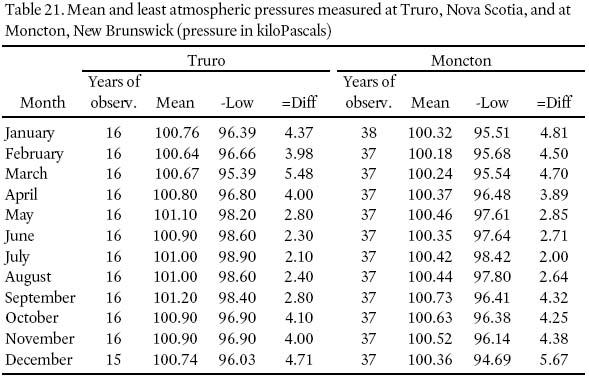
Display large image of Table 21
313 Sea level also may be raised above normal due to a wind/ storm "set-up" (see Fig. 63). This is a flow of air that drives the water toward the shore line. Here the gradient of the water is balanced by the shear stress of the wind blowing over the water. Quite apart from the set-up which propagates into the Bay due to wind over the Gulf of Maine and Scotian Shelf, in the upper reaches of the Bay of Fundy the tides (here, in reference to total water level; i.e., tide plus storm surge) are large and at times the currents are very strong. Currents in the Minas Channel can run at the rate of 7 to 8 knots (3.5 to 4 ms -1), while in the Minas Basin and Chignecto Bay the rates drop to 2.5 to 3 knots, increasing again in Cobequid Bay and Cumberland Basin to over 4 knots. Winds blowing against the current will, in effect, lessen the height of the tide and the rate of the current, but they may create tidal rips in which the surface waves are steepened to the point of breaking, causing violent seas.
Fig. 63 Storm set-ups at Charlottetown, Prince Edward Island, and at Pictou, N.S., 8 December, 1968, clearly illustrate the markedly different levels in observed tides compared to levels predicted on the basis of astronomical relations between Sun, Moon and Earth. At both localities, observed tides have a greater range than predicted tides during the surveyed 5 day interval of storm set-up.
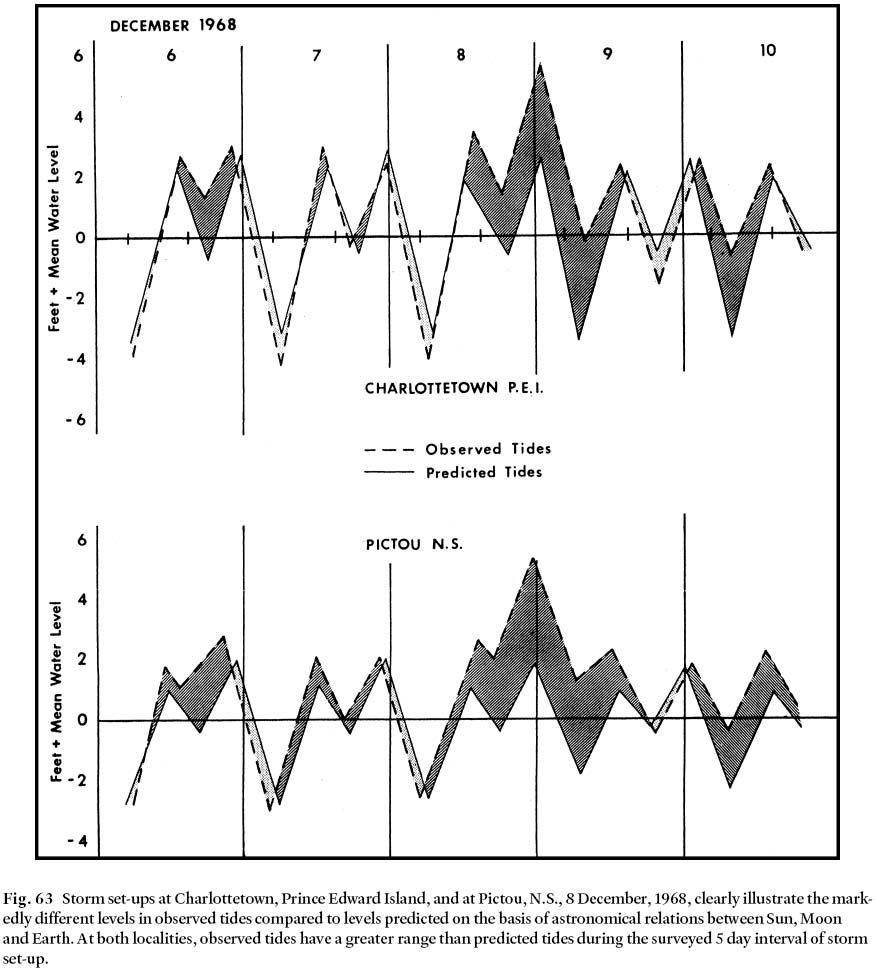
Display large image of Figure 63
314 The wind set-up is estimated by an equation which takes into account wind speed, fetch, angle between wind direction and direction for which the set-up is calculated, and the depth of the section of water. For each section with a different depth a separate calculation is made. After passing over all sections, the total wind effect will depend upon the fetch (distance over water that the wind is active). The following equation can be used to estimate the wind set-up (Sx) along the shoreline:

315 When the set-up becomes 10% of the depth, which happens when the wind speed exceeds approximately 60 times the depth in m, (55) results in too large values of Sx. It is better replaced by:

316 In areas where the tidal range is small, storm conditions can raise water levels somewhat above that of ordinary tides. In the upper reaches of the Bay of Fundy the difference between levels reached during large tides and small tides may exceed 4 m, and wind set-ups occurring during larger tides may cause flood conditions. Severe flood conditions are virtually guaranteed when adverse weather conditions coincide with the High Water of extremely large, astronomically-caused tides. The probability of such a coincidence is small and very difficult to estimate. However, indications are that in the Maritime Provinces of eastern Canada such conditions have occurred at intervals of more than a century. Historical accounts document two occasions when great storms coincided with a very high tide. These occasions were October, 1869, and November, 1759.
10.3. THE SAXBY TIDE, 1869, A PREDICTION FULFILLED
317 On the afternoon of 4 October, 1869, Thomas Earle tried to leave Beacon Light at Sand Point in Saint John Harbour (Fig. 64), but heavy seas drove him back. As wind and waves continued to rise, water flooded the first floor of the lighthouse, and threatened to rise higher. Waves broke over the top of the lighthouse, carrying away the bell and smashing the windows and the globe protecting the gas light. Retreating to the middle story, the keeper closed the hatchway behind him. The gas light continued to burn, and fanned by the storm, ignited the superstructure. In desperation Earle managed to fit a spare globe around the light, and was somehow able to contain the fire. Three and a half hours later the tide receded sufficiently to allow him to gain the safety of higher ground.
Fig. 64 An old postcard image of Beacon Lighthouse at Sand Point, N.B. (now the terminus of the Canadian Pacific Railway at Saint John Harbour), which replaced the first Beacon light, which was destroyed by fire two years before the Saxby Tide. Beacon Lighthouse was declared surplus, and destroyed in 1913.

Display large image of Figure 64
318 Thomas Earle, like most coastal folk along the Bay of Fundy, was used to high tides. He would have known the difference between "spring" and "neap" tides. He knew too that storms can cause unusually high water levels, especially when coincident with an otherwise normal high tide. Normally he would have relied on the Farmers' Almanac to predict tidal conditions throughout the year. But conditions in the Bay of Fundy on 4– 5 October, 1869 were not normal.
319 Earle may never have heard of Pliny the Elder, or of Sir Thomas Herschel, who in 1860 helped sustain the legend of 120 foot-high tides by repeating the myth of the 4th Century BCE navigator, Pytheas. However he probably had read in Maritime newspapers about S.M. Saxby's dire prediction of the great storm from which he was to only narrowly escape. The prediction had been published the previous November in the British newspapers London Standard and London Press (Saxby 1868). It read: "I now beg to state with regard to 1869 at 7:00 a.m., October 5, the Moon will be at the part of her orbit which is nearest the Earth. Her attraction, will be therefore at its maximum force. At noon of the same day the Moon will be on the Earth's equator, a circumstance which never occurs without marked atmospheric disturbance, and at 2 p.m. of the same day lines drawn from the Earth's centre would cut the Sun and Moon in the same arc of right ascension (the Moon's attraction and the Sun's attraction will therefore be acting in the same direction); in other words, the New Moon will be on the Earth's equator when in perigee, and nothing more threatening can, I say, occur without miracle. With your permission, I will, during September next (1869) for the safety of mariners, briefly remind your readers of this warning. In the meantime, there will be time for repair of unsafe sea walls, and for the circulation of this notice throughout the world."
320 Saxby, a civilian instructor of Naval Engineers of the British Royal Navy, published books and almanacs of weather predictions, claiming a relationship between stormy weather and the Moon crossing through the plane of the Earth's equator. As this occurs every two weeks it could be said that Saxby gave himself a better than 50 percent chance of claiming reliable forecasts. Note that Saxby did not specify the location where his threatening tide would occur. Astronomic conditions were to be right for higher than normal tides, world-wide, on 5 October, 1869.
321 The prediction was fulfilled in the Bay of Fundy by what was to become known as the "Saxby Tide" or "Saxby Gale". A storm hit the North American eastern seaboard on 4 October, 1869. All along the New England coast severe flooding and wind damage occurred. Between Washington and the upper reaches of the Bay of Fundy, more than 150 vessels sank or were blown ashore, 121 of them between St. Andrews, N.B., and Machias, Maine. Near Point Lepreau, N.B., the barque Genii was wrecked and eleven lives lost (Ganong 1911; Tibbets 1967).
322 At 17:00 hours, the wind increased to a gale, and an hour later rain began. By the evening of 4 October, Saint John streets were littered with debris torn from buildings. The gale continued from the south, reaching hurricane force about 21:00 hours by which time the rain had stopped. Around 22:00 hours the wind shifted to the southwest and subsided. Fully an hour and a half before the tide ordinarily would have reached its peak, waves from the Bay of Fundy were breaking over every wharf in Saint John Harbour. Ships parted from their moorings; some were driven ashore, others were badly damaged. Dozens of wharves, fish shacks, and abutments were washed away (MacLean 1979).
323 About 160 km northeast, at the head of the Bay of Fundy, the Saxby Tide occurred at 01:00 hours, 5 October, overtopping the dykes by at least 0.9 m. In Cumberland Basin, two fishing schooners were lifted over the dykes of the Tantramar marshes and deposited five kilometres from the shoreline. At Moncton, N.B., the water rose nearly 2 m above the next highest tide on record. On the marshes west of Amherst, N.S., a barn in which some people had been sleeping, was despatched well over a kilometre up the marsh. During the course of the storm two men were carried out to sea and drowned. Three others were able to cling to timbers and were eventually washed ashore. Much of the hay stored on the marsh was swept out to sea and the remainder was scattered over the area. Farmers drew lots in order to divide the little hay that was salvaged. In and around the Minas Basin, the gale was less severe, although the rainfall was heavy. Everywhere dykes were breached, cattle and sheep were drowned, lengthy portions of railroad beds were washed away, and in many areas travel became impossible. Communications likewise were shut down by the weather to a degree difficult to imagine today.
10.4. HEIGHT OF THE SAXBY TIDE
324 A year after the disaster, a survey was made between 13 August and 31 December for a proposed canal across the Chignecto Isthmus from the Bay of Fundy to the Northumberland Strait. To simplify calculations, by avoiding negative values, the surveyors assumed a datum (reference elevation) of 100 feet (30.48 m) below the average top elevation of the dykes. By this reckoning the Saxby Tide was reported to have reached levels of 100 feet or more. These figures of course have no direct relationship to mean sea level. But they have, unfortunately, helped perpetuate the erroneous notion of enormous tides.
325 During the 1870 survey, extremely high astronomical tides (i.e. tides not associated with storms) occurred on 23 September (28.83 m), 26 October (28.83 m), and 23 November (28.80 m) for an average of 28.82 m. Comparing this elevation with the average top elevation of the dykes yields (30.48 m– 28.82 m) a difference of 1.79 m. Thus although the level of the dykes may have been raised slightly in the years since 1870, the Saxby Tide was at least 1.5 m higher than astronomically caused high tides.
10.5. THE STORM TIDE OF 1759
326 Only sparse accounts survive of a probable precedent, over 100 years earlier, of the Saxby Tide. The nameless historical storm tide battered the Bay of Fundy region on 3 and 4 November, 1759. In Beamish Murdock's "History of Nova Scotia" contained in the Gentleman's Magazine of 1760, it is recorded that at Fort Cumberland (earlier and later named Fort Beausejour) 700 chords of firewood were swept away from a woodyard that was at least 3 m above the protecting dyke. In Saint John Harbour water reportedly rose 1.8 m higher than was usual for large tides. Storm waves broke on the terraces of Fort Frederick, located well inside the Harbour, demolishing a store house and spilling provisions into the sea.
327 It is unknown whether anyone foretold the historical storm tide of November 1759. The regionality of storms and storm tides makes predictions like Saxby's a rather unscientific exercise, however much they may impress the local populace. Even today, meteorologists, assisted by a world-wide computerized network of data-gathering instruments on the ground and in satellites, are faced with more variables than they are able to handle (Wells 1986). The behaviour and frequency of complex extraordinary weather systems, their whereabouts, strength, rate and direction of movement, are beyond their grasp.
10.6. THE GROUNDHOG DAY STORM, 1976
328 Whereas the Saxby Gale was predicted a year before it happened, the "Groundhog Day" storm of 2 February, 1976, was forecast only hours before it broke. Two days earlier a weak low pressure area hovered over Alabama and Texas. Subsequently, this system met a small high pressure system from western Ontario. Small craft warnings were issued on 1 February, advising of strong southerly winds. Then around noon that day, gale force winds were predicted. During the night, gale warnings were changed into severe storm warnings. By 8:00 hours on 2 February, the barometric pressure had dropped precipitously over the Gulf of Maine, signalling the likelihood of a storm accompanied by higher than normal tides (Amirault and Gates 1976).
329 The storm hit the coast of Maine hard (Morrill et al. 1979). In places, the tide rose more than 2.5 m above the predicted level, heavily eroding the coastline. Waves hammered coastal installations. A freighter anchored in Penobscot Bay was blown aground. The strong south-southeasterly winds, which had been blowing for 5 to 6 hours over the open water along the major axis of the Penobscot Bay, resulted in a storm surge in the Bay and up the Penobscot River. Much of Bangor was flooded. In less than 15 minutes the water reached its maximum depth of 3.7 m in the river, 3.2 m above the predicted tide level.
330 By the afternoon of Groundhog Day (2 February, 1976), the storm was raging along the eastern seaboard (Fig. 65). Intermittent power failures and curious sparking effects were the result of short circuits caused as winds swept seawater across the countryside. Fortunately, the tide was an apogean spring tide (Conkling 1995). In Saint John, the high tide was expected to be only 7.7 m (25.2 ft) above CD at 13:10 hours. Note that for comparative purposes, this is almost exactly equal to mean Higher High Water (25.3 ft) at Saint John. However, on the afternoon of Groundhog Day the tide rose to 9.16 m (29.65 ft) above CD, fully 1.46 m higher than expected. The damage would have been simply enormous had the storm occurred on the perigean spring tides: sixteen days later on 18 February, the tide at Saint John was predicted to reach a height of 8.4 m above CD; a month and a half later, on 18 March, the tide was predicted to rise 8.66 m above CD; two and a half months later on 16 April, the tide was predicted to be 8.84 m above CD, 1.07 m higher than the predicted tide on Groundhog Day. In short, a storm on 16 April, 1976, would have had the potential of causing calamity on the scale of the Saxby Tide.
Fig. 65 In the aftermath of the Groundhog Day storm of 2 February, 1976, the streets and waterfront of Saint John, N.B., were in a shambles. Photograph courtesy of Saint John Telegraph Journal.

Display large image of Figure 65
331 In light of the above considerations it seems a distinct possibility that another storm tide of the magnitude of the Saxby Tide of 1869 will occur in the Bay of Fundy region. The big question is when will this storm likely occur? Until then, successor dykes to those erected during the 17 th Century along the Bay of Fundy marshlands, continue to protect agricultural lands.
332 These agricultural lands are shrinking before the onslaught of modern highway and suburban development schemes, not to mention the continued transgression of the sea. Aboiteaux draining these lands are of course unable to discharge when the tide outside is higher than the water upstream. With a heavy runoff, the potential therefore exists for the land to be flooded with fresh water. This is realized and tolerated by farmers of course, but the situation is rather less stoically accepted by developers.
333 Generally, the stronger tides happen during spring and summer around midnight, and during fall and winter near noon. But the fact that the Saxby Tide occurred during the night and in the fall shows that even this rule is not valid for extraordinarily severe storm tides. Nor does the fact that the landmass of the upper Bay of Fundy area is submerging at a rate of about 3 mm per year improve the situation. The dykes can be made higher, but if they are not raised to Saxby-type levels, their overflow will raise the flood levels in the dyked areas that much higher. The developed areas near Truro, Weymouth and Advocate in Nova Scotia, and Moncton in New Brunswick (see Fig. 60), are among potential victims of such storm tide events.
11. Periodicity of the Tides (TOP)
11.1. INTRODUCTION: THE SAROS CYCLE
334 Pytheas, a navigator from the Greek colony of Massalia (modern Marseilles, France), explored the northern Atlantic Ocean in the Fourth Century B.C.E. Proceeding north after passing between the Pillars of Hercules, he noticed the lengthening of the summer days and observed the midnight Sun in Thule, a six day voyage north of Britain. He was aware too, of the relationship between tides and the Moon's motion along its orbit.
335 Pliny the Elder (23– 70 A.D.) mentioned in his Historia Naturalis that, according to Pytheas, the tides north of Britain rise to heights of 120 feet (" octogenis cubitis"). The notion of the existence of such enormous tides persists. For example, the eminent 19th Century scientists Sir John Herschel and Sir Oliver Lodge repeated the belief that 120 foot-high tides occur in the Bay of Fundy. Only a few years ago the same misconception was linked to the extraordinarily high tides associated with the so-called "Saxby Gale".
336 One might wonder where the extraordinary high tides occurred that so impressed Pytheas. He must have been familiar with the 40 foot-high (12.19 m) tides that regularly occur along the Brittany coast on the French side of the English Channel, or in the Bristol Channel south of Wales. According to the Roman writer Festus Avienus, these waters were visited a century before by Himilco, a famous Phoenician explorer, and by merchantmen trading for tin. The only other tides in the North Atlantic of the same order of magnitude are the 30 ft (9.14 m) tides in the White Sea portion of the Arctic Ocean, and the more than 40 ft (12.19 m) tides in Ungava Bay, Quebec and the Bay of Fundy. The White Sea can only be reached by waters lying north of the Arctic circle where the midnight Sun can be observed in midsummer. Could Phoenician seafarers have reached the western side of the Atlantic and, after visiting the Bay of Fundy, passed to Pytheas the notion of 120 foot-high tides?
337 As we have seen, tides are caused by the attraction of the Moon and Sun on water particles near the surface of the Earth. Since the orbits of the Moon around the Earth, and of the Earth around the Sun, are elliptical, the effects are variable in strength, like the resulting tides. The redeeming feature is that every aspect of each motion has a corresponding periodicity to which tidal variations can be related. The pages-long equation describing the paths of celestial bodies, a masterpiece of human ingenuity, was first set out by Louis Lagrange (1736– 1813) and Pierre Simon de Laplace (1749– 1827). Yet even the ancients possessed considerable knowledge concerning these matters.
338 Nearly four centuries before Pytheas described the influence that the Moon's motions have on the tides, Chaldean priests in the Middle East were able to predict recurrence of eclipses. This was because of their knowledge of the Saros, a Babylonian name adopted by modern astronomers for a cycle with a period of 18 years, 11 days and 8 hours. In this 18.03-year cycle, the Moon, Sun, and Earth return to almost identical relative positions to each other. This is the cycle in which similar solar and lunar eclipses repeat themselves. Eclipses result when the Sun, Moon, and Earth are in, or almost in, one straight line.
339 The paths of the solar eclipses over the Earth's surface are almost identical in shape, but are located 110° to 130° west of the path of the eclipse of 18 years previous (Abell et al. 1988). For example, one series of solar eclipses began on 17 May, 1501 (Julian calendar), as a partial eclipse. (At present, 12 such series producing total solar eclipses occur during a Saros cycle of 18.03 years). After 15 Saros cycles with partial and annular eclipses, the eclipse became total on 6 November, 1771. The total eclipse seen on 7 March, 1970, over Mexico, the USA and Canada was one of the series; likewise that of 18 March, 1988 as seen over the Pacific, Sumatra and Borneo (see Fig. 66). After this, there will be 35 more total eclipses followed by half a dozen partial ones. All told, the Saros prediction is valid for 1226 years [(1988– 1501) + (35+6) · 18.03 = 1226.23 years)] for this particular series.
Fig. 66 Total solar eclipses by month and year from 1970 through 2030 A.D. Note the 18.03 year Saros cycle, after which time Moon, Sun and Earth return to almost identical positions relative to each other. At present, 12 total solar eclipses occur during a Saros cycle of 18.03 years.
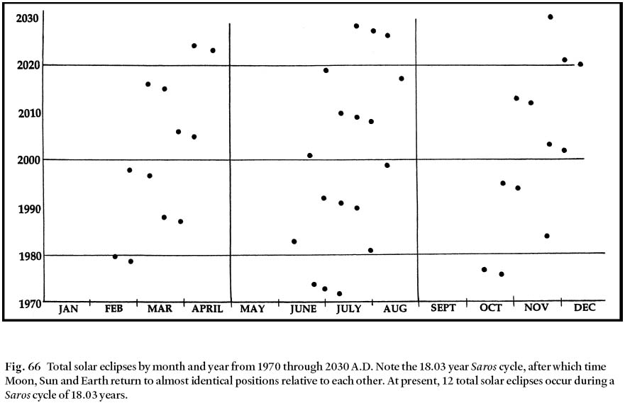
Display large image of Figure 66
340 Because the astronomical conditions conducive to generating large tides match the Saros cycle, their recurrence at 18.03 year intervals is expected. Could it be that this particular timing is closely linked to the occurrence of exceptionally high tides like the Saxby Tide? There is good suggestive evidence that this is the case, but first we need to look further into the causes of tides and their variations. Only then will we better appreciate the implications of the Saros for a future tide comparable to the Saxby.
11.2. ASTRONOMY AND THE VARIATIONS OF TIDES
341 Orbital forcing of tidal cycles is only a small portion of the spectrum (Fig. 67) of astronomically-driven periods which exert gravitational effects on Earth and the affairs of humankind (Rampino et al. 1987). The same periodic behaviour governs changes over time in the energy distribution reaching Earth's atmosphere, and must have done so throughout geologic time. We are concerned here only with tidal phenomena within a small portion of the calendar and solar frequency bands.
Fig. 67 Orbital forcing time scales (logarithmic) of tidal cycles is only a small portion of the spectrum of astronomically-driven periods which exert gravitational effects on Earth and human affairs. Modified from House (1995).
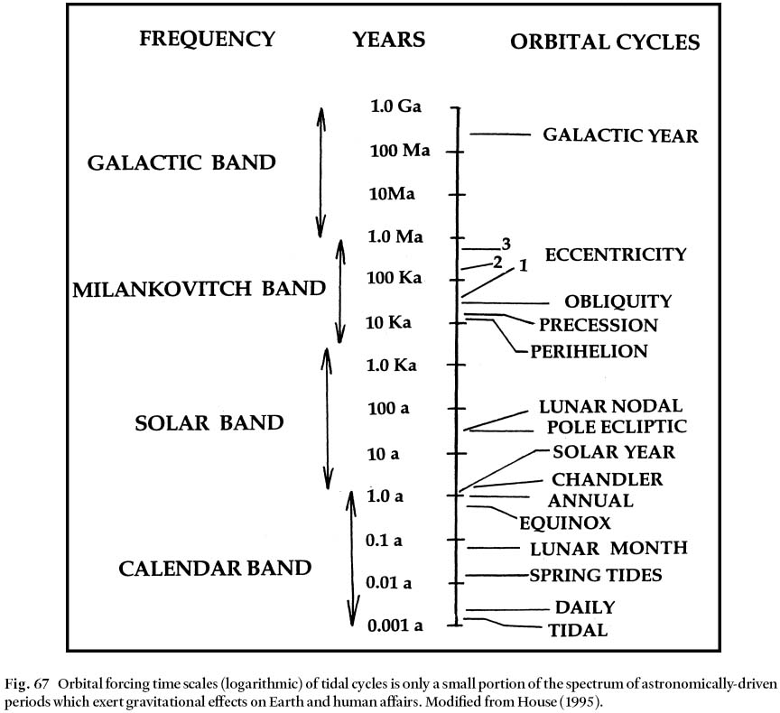
Display large image of Figure 67
342 S.M.Saxby might have added to his prediction that the great storm tide destined to immortalize him, especially in the view of many Maritimers, would coincide with the Saros (Desplanque 1974). In this 18.03 year cycle, Moon, Sun and Earth return to almost identical relative positions. It is astounding to realize that by 800 B.C., Chaldean priests knew the Saros well enough to accurately predict eclipses. Could it be that eclipses, or more particularly the time interval between eclipses, might be associated with far higher than normal tides?
343 In general, the average gravitational effect of the Sun is about 46 percent that of the Moon; however, in the Bay of Fundy the effect of the Sun is only about 15 percent that of the Moon. Further, because the orbits of the Earth around the Sun and the Moon around the Earth are elliptical, and their paths influenced by many factors (Fig. 67), the gravitational effects are variable in strength, like tides (House 1995).
344 Normal tides are termed astronomical tides because their main variations are generated by three astronomical phenomena as noted earlier: the variable distance between the Moon and Earth; the variable positions of the Moon, Sun and Earth relative to each other; and the declination of the Moon and Sun relative to the Earth's equator. Additional astronomical factors that influence tides include: the Earth's rotation; the eccentricity of the Moon's orbit, which varies depending on the Sun's position in relation to the longest axis of the Moon's orbit.
345 Non-astronomical phenomena include: the possible increasing tidal range in places like the Bay of Fundy due to deepening waters (Godin 1992); atmospheric disturbances; the geometric shape of inlets, bays and ocean basins; the postglacial rise in sea level (see Fig. 68). This last factor, by no means trivial, translates to about a world-wide 2 mm/yr submergence of the land in relation to sea level (Schneider 1997).
Fig. 68 Triangular diagram shows the relative importance of the main astronomical and non-astronomical phenomena that contribute to the generation of storm tides in the Bay of Fundy.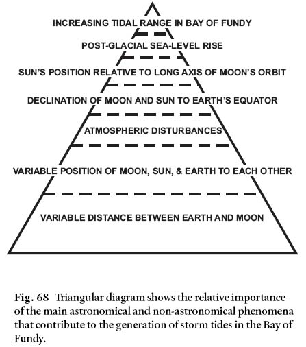
11.3. THE LARGEST ASTRONOMICAL TIDES
346 As seen from Earth, the Moon and Sun seem to move within two imaginary rings around Earth's centre (Fig. 69). The ring in which the Moon's motions are confined has an outside diameter of 813 000 km and a maximum thickness of 50 000 km, while its width varies during an 18.61 year period between 410 000 km and 255 000 km. The Sun appears to move within a similar ring, with an outside diameter of 3.04 · 10 8 km, a maximum thickness of 5 · 10 6 km, while its width remains constant at 1.25 · 10 8 km. At perigee the distance to the Moon is 3.57 · 10 5 km, and at apogee the distance is 4.07 · 10 5 km.
Fig. 69 This diagram indicates the variation in the obliquity of the Moon's orbit during the nodical lunar cycle, completed in 18.6 years; this introduces an important inequality in tidal movements. The angle β#xDF;, between the ecliptic and the celestial equator (the obliquity of the ecliptic) has a nearly constant value of 23.5°. Angle i, between the ecliptic and the plane of the Moon's orbit has a value of about 5°. Angle I, the obliquity of the Moon's orbit, measures the inclination of the Moon's orbit to the celestial equator. Its magnitude changes from 18.5° to 28.5°, with the position of the Moon's node. When the Moon's ascending node N, coincides with the vernal equinox, I = β#xDF; – i = 18.5°. After Schureman (1941, p. 6).
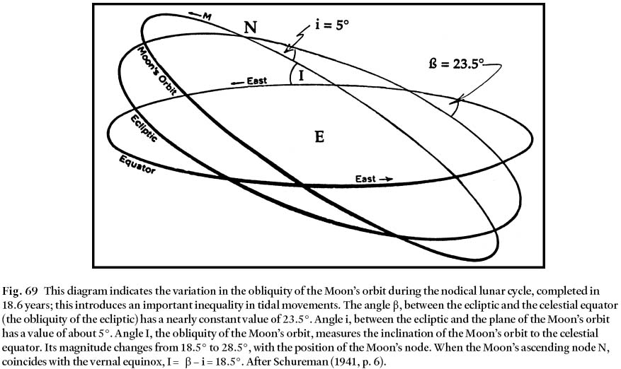
Display large image of Figure 69
347 The positions of the Sun and Moon in their respective (elliptical) orbits, and in relation to each other and the Earth, are only occasionally repeated. When one position is inducive to generating large tides, an approximate date for a repeat performance can be determined by matching the several types of astronomical months. Such months are designated as synodic, anomalistic, tropical, nodical or evectional, according to whether the revolution of the Moon around the Earth is relative to the Sun's position, the shortest distance to the Earth, its passing through the Earth's equator, its passing through the ecliptic, or the variation in the eccentricity of its orbit. For some months, such as the synodical (full and new moon), tropical, and nodical, the characteristics influencing the tides occur half-monthly. Since the synodical conditions provide the dominant tidal conditions, one can expect two sets of spring tides during one synodical month. But when one of these sets coincides with the Moon's closest approach to the Earth, extra high (perigean) spring tides will occur.
348 It takes 29.531 solar days between one new moon and the next. However, only 27.555 solar days (anomalistic month) elapse from the time that the Moon is closest to the Earth, to the next such occasion during the Moon's elliptical orbit around Earth. When the Moon is in perigee, and its phase is either full moon or new moon, one can expect the strongest tides. However, as the periods of both movements are not the same, the coincidence of such occurrences is only periodic.
349 Imagine a racetrack. On this track are two cars, marked N and F. They always move half a track apart around the raceway. Let the raceway be 360° long. Thus, each day, these cars move 360°/29.531 = 12.19°/day (V). Another car, marked P, starts at the same time beside car N, but its velocity is 360°/ 27.55 = 13.06°/day (W), thus somewhat faster than car N. In time, car P will overtake car F, which was 180° in front of car N. The time it will take to close this gap can be calculated (approximately) as 180/(W– V) = 205.892 days.
350 The same applies to lunar movements. After about 206 days, the conditions for stronger than average tides recur, perigee coinciding either with new moon or full moon. Two of these periods are 411.78 days long. Thus, each year one can expect the conditions for stronger tides to be (411.78– 365) = 47 or 46 days (leap year) later than in the previous year.
351 The declination of the Moon also has an influence on the strength of the tides on particular days. This declination has its strongest values twice in a period of 27.321 solar days (tropical month) with a velocity of 360°/27.32 = 13.18°/day. This is somewhat faster than the velocity of the perigee. Therefore in order to have the coincidence of a similar combination between perigee and declination of the Moon, it will take 1615.75 days, or 4.42 years. Should a particular part of the declination cycle cause somewhat higher tides then the coincidence with perigee will repeat after 4.42 years. During the Saros cycle of 6585.32 days, there will be 238.997 perigee cycles, 446.01 (full moon-new moon) cycles, and 482.07 declination cycles.
352 The most favourable combination of factors to produce strong tides in the Bay of Fundy occurs when perigee coincides with spring tide at the very time that anomalistic, synodic and tropical months peak simultaneously. As it happens (see Table 22), the best match occurs after a period of 6585.3 days (18.03 years). The driving mechanism of this cyclic phenomenon is the same one that orders the timing of eclipses – the Saros.
Table 22. Long term cycles of astronomical conditions leading to stronger or weaker than normal tides
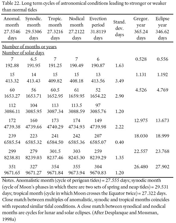
11.4. COINCIDENCE OF STORM TIDES WITH SAROS
353 Given the clockwork precision of astronomical conditions and their absolute control over normal tide variations it is reasonable now for us to enquire whether the Saxby Tide, and for that matter other historical storm tides in the Bay of Fundy, coincided with the Saros.
354 What are the chances of a periodic storm system on the scale of the Saxby tide? The only certainty is that the relationships between the Moon and the Sun that produce the highest tides on Earth are repeated in the same periods as those that create solar and lunar eclipses (Abell et al.1988), namely the Saros cycle of 18.03 years. Therefore, to check the position of an historical high tide in the Saros, one need only add to the tide's date the appropriate multiple of the Saros (Table 23) to reach a particular time interval for which the tidal record is well known. Detailed tidal records in Canada were first kept about 1894. So as a reference point let's choose a date close to the end of 1958, which is eleven Saros after the Saxby Tide. The tidal levels referred to are those measured at Saint John, where the average high tide is 7.7 m (25.2 feet) above CD. To test the reliability of the method of prediction, our examples of historical storm tides can now be checked against predicted tides, n Saros cycles later.
Table 23. Multiples of the Saros
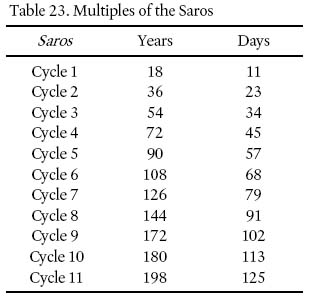
Display large image of Table 23
355 Checking the multiples of the Saros against storm tides, we discover that the storm tides of 1759 and 1869 correlate very closely with predicted high tides of the Saros cycle (Table 24). So do the 1976 Groundhog Day storm, and the exceptionally High Water of 12 October, 1887, experienced in Moncton, and the storm tides of 20– 22 December, 1995 (Taylor et al. 1996). However, it is important to bear in mind through any exercise of this type that Saros cycles are long term harmonic motions. This means that near the top or bottom of the cycle the rate of change with time is relatively small. Thus, the "peaks" of Saros cycles are not confined to points in time, but to rather short intervals of time.
Table 24. Countback of tides in the Bay of Fundy at 18.03-year intervals
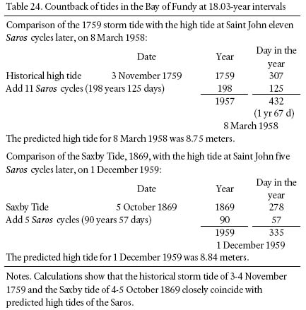
11.5. PROBABILITY OF A REPEAT OF THE SAXBY TIDE
356 Whether property owners along the Bay of Fundy should be reminded of their next appointment with the Saros in 2012– 2013 AD is not trivial question (Fig. 70). With increasing encroachment of people in coastal zones, the risk of loss of life and major property damage in the Gulf of Maine-Bay of Fundy region is substantial in the event of a tide like the Saxby Tide (Shaw et al. 1994). Simply put, what is the probability of a storm tide coinciding with a large astronomical tide? We can conveniently address this question using the above examples. We know that a "peak" of the Saros occurred between 6 March, 1958, and 31 December, 1959. During this time, there were 1288 tides at Saint John, 37 of which were extreme astronomical high tides (28.5 feet or higher). Thus, the chances that an historically memorable storm tide coincided with one of the 1288 tides, is slightly less than 3 percent. This is assuming that the occurrence of stormy weather conditions is spread evenly throughout the year. The increased incidence of high winds during late spring and fall probably favours the odds of gale force conditions coincident with high tides slightly above 3 percent.
Fig. 70 Crossing the Tantramar Marsh during High Water, spring tide, 9 November, 1980, looking northwest from Aulac, N.B. The closest Saros date was 12 December, 1978, a year of many high waters. Photo by Elly Desplanque.
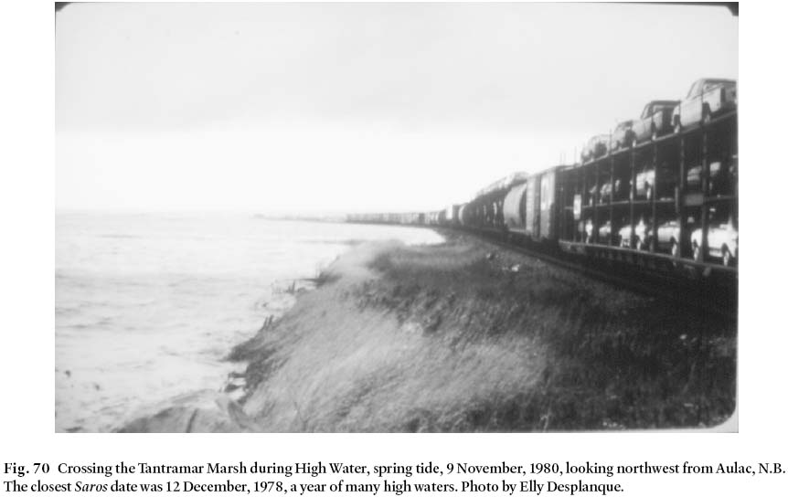
Display large image of Figure 70
357 Most assuredly, postglacial sea-level rise is a significant factor in all this. With each and every repeat of the Saros, an increase of the high tide mark of at least 3.6 cm (2 mm/year for 18 years) can be expected. Thus, since the Saxby Tide more than seven Saros ago, sea level has risen eustatically nearly 25 cm. Added to the minimum 1.5 m by which the Saxby Tide exceeded high astronomical tides, a height is calculated that that is more than sufficient to overrun the present dyke system.
358 It seems likely that tides like the Saxby might be recurrent, although one wishes for a larger database. The clockwork precision of astronomical conditions exerts absolute control over normal tidal variations. But there remains much to learn about long term periodic events associated with tides and the weather. We have seen that only significant storms coincident with large tides, or extraordinarily severe storms coincident with medium tides, can result in higher tide marks than are reached by astronomical tides alone. Detailed tidal records over several decades show that in the Bay of Fundy there is a tendency for slightly higher maximum monthly High Water marks in a 4.5 year cycle, examples being the peaks that occurred in 1998 and 2002. Indeed, in this region, high perigean tides levels can be anticipated at intervals of 1 month, 7 months, 4.5 years and 18 years. When such high tide levels coincide with severe atmospheric disturbances, exceptionally High Water surfaces can be expected. However, short of an extraterrestrial catastrophe, they are not likely to attain the 120-foot (36.6 m) height of legend. Property owners along the Bay of Fundy should nevertheless keep in mind their next appointment with the Saros in 2012– 2013.
12. Tidal Boundary Problems in the Coastal Zone (TOP)
12.1. INTRODUCTION: CAVEAT EMPTOR!
359 The need for precise determination of tidal water boundaries stems from numerous concerns, including cadastral surveying, coastal property evaluation, development of offshore resources, protection of fisheries, and ownership of the foreshore and sea bed (Nichols 1983; Daborn and Dadswell 1988). Historically, the dividing line between wet and dry land, or as far as the tide ebbs and flows, has been critical in resolving tidal boundary problems in the coastal zone (Ketchum 1972). However, the location of the mean high water line has been a matter of considerable litigation (Greulich 1979; Desplanque 1977). What exactly is this dividing line, and how can levels like Mean High Water and Mean Low Water be most accurately defined?
360 Presumably, Mean High Water is reached under mean astronomical conditions, with perhaps some long-term tectonic and climatological influences to be considered. Climatic influences in Atlantic Canada tend to raise the water during the winter months, so that in areas of relatively small astronomical tides along the Atlantic seaboard the frequency of extreme high observed water levels is higher during that season. However, astronomical influences are variable and follow cycles in which the magnitude of influences waxes and wanes (Schureman 1941). The longer the cycles, the greater the variation. In the Fundy region, as discussed earlier (section 11.0), distinct cycles are recognized (Desplanque and Bray 1986).
361 Meteorological influences can raise or lower water surface levels over a period of days, during which time High Waters and Low Waters are similarly affected. On a year long scale, climatic influences in the Atlantic region tend to raise the water level during winter months. Thus in areas of relatively small astronomical tides along the Atlantic coast of North America the frequency of extreme high observed water levels is higher during winter. The eustatic rise of sea level can not be neglected in these considerations: over the course of an 18 year cycle, accepting a global average 2 mm/yr eustatic rise in sea level (Schneider 1997), water level will have risen by about 3.5 cm. In view of the above considerations it appears that decisions handed down in courts of law on issues concerning tidal water boundaries are in many cases equivocal (Nichols 1983; Desplanque 1977).
362 Harvey et al. (1998) provided a very interesting analysis of the legal and policy framework concerning the restoration of the habitat of Fundy estuaries. Unfortunately, important overlapping boundaries of provincial and federal jurisdiction, in some cases unresolved, seem to have resulted in poorly regulated environmental protection. Details of the many issues of territorial and legislative jurisdiction, as they generally concern Bay of Fundy waters and the coastal zone, are beyond the scope of this paper. Nevertheless many of the key issues center on the problem of establishing specific water level boundaries.
12.2. MEASUREMENT OF TIDAL LEVELS
363 Concerning the tide levels and terms used in Canada (as set out in section 2.1), all tidal measurements are made from the local Chart Datum (CD). The International Hydrographic Bureau recommends that CD at a certain location should be at an elevation so low that the tide at that place will seldom if ever fall below it. The reason for this recommendation is that the soundings on hydrographic charts will show the minimum depth of water with which mariners will need to deal. The tidal range gives them an extra margin of safety. Generally tidal range is small and so is this factor in their margin of safety. However, on Bay of Fundy charts showing a number of tidal stations, the difference between CD and Mean Water Level (MWL) in one section of the charted area may be quite different than it is in other sections. The soundings on such charts do not allow one to construct a proper three-dimensional picture of the shape of the Bay.
364 The Canadian Marine Sciences Branch defines mean sea level (MSL) as the level that oceanic water would assume when no atmospheric, hydrologic or tidal influences act upon it. They also use the term Mean Water Level (MWL), which is the sea level resulting in the absence of tidal influences. Up to certain limits the base level of the tides is moving up and down with the water level caused by atmospheric and hydrologic conditions. Since it is easier in the field to establish a local MSL or MWL than a level indicating the Mean High Water Mark (MHW), it is recommended that MHW be the level reached by the M2 amplitude above MSL.
365 It is worth noting too that whereas the Canadian Tide and Current Tables give the values of tidal differences for Higher High Waters and Lower Low Waters, the U.S. Tide Tables give the values for Mean High Water (MHW) and Low High Water (LHW). Consequently, the values of the ranges for mean and large (spring) tides differ greatly in both tables for the same locations (see Table 25). The differences between these datums are significant to the problem of establishing tidal boundaries. Canada apparently lacks a definition of MHW, a level usually taken in surveying practice as equivalent to "Ordinary" High Water (OHW) (Nichols 1983). Britain's intertidal zone is also proving difficult to map due to use of different vertical scales by Ordnance Survey and the Admiralty's Hydrographic Office, and the fact that the latter organization uses "the lowest astronomical tide" as zero point for depth (Tickell 1995). The Americans take MHW as the average of all the High Water heights observed over the National Tidal Datum Epoch. For this reason American definitions are inappropriate for direct use in Canada.
366 Next let's examine how an accurate determination of the Mean High Water mark can be made.
Table 25. Comparison of Canadian and American Tide Tables (1975) of tidal ranges for the same six selected ports
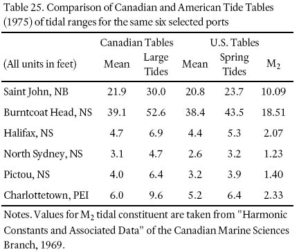
12.3. TIDE PREDICTION: MEAN SEA LEVEL AND MEAN HIGH WATER
367 For most locations (ports) along the Canadian sea coast, the M2 tidal constituent is dominant. In fact the amplitude of the M2 tide very closely represents the average tidal conditions. When measured above the local MSL, it will indicate the level of MHW. The value of this amplitude has been determined for a great many ports along the Canadian sea coast. As for MSL, it can be easily determined by taking the average of hourly readings in calm conditions over one lunar day. The mean of these readings should indicate the MWL of the day. In order to verify if this level is close to MSL one can check at the nearest tidal recording station if the observed tides for that day correspond closely to the predicted ones. If so, the MWL can be used as a substitution for MSL. Otherwise a correction can be made by applying the difference to the measured value of MWL. Generally these differences (when they occur) are in the same order of magnitude for a number of recording tidal stations.
368 Since the Higher High Water (HHW), the Lower High Water (LHW), and the MWL values (see Table 26) above local CD are determined for a great number of stations along the eastern seaboard, the Mean High Water mark for most locations can be accurately determined with very little effort. A large degree of accuracy is not warranted because the landmass of the southern part of the Atlantic Provinces is steadily submerging at a rate matched by the rise of the High Water mark.
Table 25. Comparison of Canadian and American Tide Tables (1975) of tidal ranges for the same six selected ports
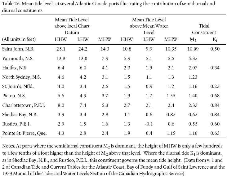
12.4. THE WATER'S EDGE: CONFUSION IN LEGISLATURE AND LITERATURE
369 As expressed in Canadian law, "The land on the seaward side of the high water mark is prima facie held by the sovereign in common law jurisdictions." In other words such land is generally owned by the state, i.e., in Canada, the provincial or federal government.
370 Some Nova Scotia acts, for example, reflect this principle (Kerr 1977). The 1967 Nova Scotia Beach Protection Act states that the Governor in Council, on recommendation of the Minister of Lands and Forests, may designate as protected beach, an area which "…may include the land extending seaward from mean high water mark and such land adjacent thereto … The Minister of Lands and Forests may post signs on or near land of the Crown extending seaward from mean high water mark, warning the public that the beach is protected under this Act".
371 The 1975 Nova Scotia Beaches Preservation and Protection Act declares that "beach" means that area of land on the coastline to the seaward of Mean High Water mark, and that land landward immediately adjacent thereto, to the distance determined by the Governor in Council.
372 The 1949 Nova Scotia Marshland Reclamation Act interprets as "marshland" the land lying upon the sea coast or upon the bank of a tidal river, and being below the "level of the highest tide". Legislative practice assumes that the vertical and horizontal location of the Mean High Water mark, and the level of the highest tide are established and available all along the coastline. Unfortunately, confusion abounds in legal circles about the characteristics of the tides and the terminology used to describe them. For instance, in the upper reaches of the Bay of Fundy the tides can reach more than 8 m above MSL during strong tides, whereas during weak tides the High Water is scarcely 3 m above that level. Approximately 50% of the tides reach above the 5.5 m mark. Furthermore, the range varies from year to year and from location to location along the coast. Complicating matters is the fact that MSL changes even in the short term (Fairbridge 1987), at different rates in relation to the landmass, depending upon the location. Indeed, the concept of MSL is like Earth's Magnetic North Pole, elusive. Thus, in tide tables, the term Mean Water Level is used.
373 The confusion in legal circles is exemplified in "Water Law in Canada-The Atlantic Provinces" (La Forest 1972) where the three types of tide of which the law takes cognizance are described:
- Tide type #1 – high spring tide, which occurs at the two equinoxes;
- Tide type #2 – spring tide, which happens at the full moon and the change of the Moon;
- Tide type #3 – the neap, or ordinary tide, which takes place between full moon and change of the Moon, twice every twenty-four hours.
374 Firstly, Pliny the Elder (23– 79 A.D.) observed that the tides appear to be the strongest in the periods close to the equinoxes, namely on 21 March and 23 September. This observation may well be true for tides along the eastern side of the North Atlantic Ocean. However, Pliny could not know that the conditions along the American coastline are different. Thus, Table 27 shows that although tides on the eastern side of the Atlantic are highest near the equinoxes, this is clearly not the case for tides along the eastern or western coastlines of North America. Note that the tides in 1953 and 1975 on the eastern seaboard of North America may reach their highest levels at any month of the year due to their advance by 47 or 46 days each year as a result of perigee coinciding with either new moon or full moon. The definition of tide type #1 implies that equinoctial tides are in a way special, but this rule is in no way universal.
Table 27. Highest monthly tides at ports along eastern and western coastlines of North America, and the eastern side of the North Atlantic Ocean in 1953 and 1975
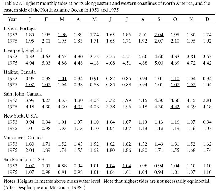
Display large image of Table 27
375 Secondly, the term "change of the Moon" is archaic, and designates new moon. It means, simply, that tides occurring during the period that the Moon appears in its full moon and new moon phases are stronger than average tides. This is of course due to the fact that these phases of the Moon occur when the Earth, Sun and Moon are most closely aligned. At these times, the gravitational action of the Sun reinforces the action of the Moon, resulting in higher than average tides, just as is supposed to happen in type #1 tides. During its orbit, the Moon is in one of its two quarter phases when halfway between its new moon and full moon positions. At such times the gravitational action of the Sun counteracts the dominant Moon's action, resulting in neap tides.
376 Unfortunately, in legal circles European tidal conditions are taken as standard and assumed to be universal. Theoretically the Sun's action is close to 46% of the Moon's gravitational influence. However, when the tides are analyzed, the actual percentage can differ depending upon the locality. Some of the measured percentages on the east side of the Atlantic Ocean are: Casablanca 37%, Rabat 40%, Lisbon 39%, St. Nazaire 35%, Flushing 27%, Bremerhaven 25%, London 27%, Liverpool 32%, Kingstown 30%. These figures are the ratios between the local tidal constituents S2 and M2 (Schureman 1941). Note that these percentages are smaller than the theoretical one. Nevertheless, they are relatively strong compared to those along the North American eastern seaboard south of Sable Island. Here the percentages are 20% or even less (15%) in the Bay of Fundy. This diminished strength of the Sun-caused tides means that the term "spring tide" loses much of its significance. In the Bay of Fundy the varying distance between Earth and Moon is the most important factor in determining tidal strength. Perigean spring tides are outstanding, while apogean spring tides hardly differ from average tides. Thus, the importance otherwise given to the term "spring tide" shows that tidal phenomena around the North American continent are not very well understood in legal circles.
377 Thirdly, the term "neap, or ordinary tide … which takes place … twice every twenty-four hours …" is a very confusing expression. For example, the period of 24 hours is not very precise because in most cases, the tides occur on average twice in a period of 24.84 hours, the lunar day. However, it is the term "neap or ordinary" that presents difficulty with respect to definition.
378 The term "High Water of Ordinary Spring Tides" is used in some British publications. The U.S. Coast and Geodetic Survey Tide and Current Glossary (1999) mentions that the term "ordinary" is not used in a technical sense by the Survey, but that term, when applied to the tides may be taken as equivalent to the terms "mean" and "average" (ASCE 1962). Thus, from that service's point of view the "ordinary tide" would be the same as the "mean tide". However a neap tide is a tide weaker than a mean or average tide. Thus the term "… the neap or ordinary tide …" is a contradiction in terms.
379 Tide type #3 is correct insofar as this tide takes place between full moon and the "change of the Moon" (new moon), and presumably is the weakest possible. However, the term "ordinary", has various meanings, one being "of common or everyday occurrence", another being "average or mean" (La Forest 1972). However, when a condition is variable, it is not possible for that condition to also happen all the time, yet be the average condition. It is also true that all tides equal to or greater than the neap tide will attain a certain common level. It could be argued that a neap tide is an ordinary tide. However, it certainly will not be a mediocre, medium, mean, normal, or average tide. In this case the weakest possible tide is set as a standard. No mention is made of the variability of the distance between the Moon and Earth although this is an influential cause of tidal variability, and of high tides, and can equal or exceed the effect of the changing phases of the Moon.
380 In order for true diurnal tide conditions to exist, the amplitude of the diurnal tide must be two to four times larger than the semidiurnal tide, depending on the time relationship between the two. However, under certain astronomical and oceanographic conditions, tides may vary from diurnal to semidiurnal during a span of little over a day. Thus only one tidal oscillation sometimes occurs in the southern parts of the Gulf of St. Lawrence and in Northumberland Strait. This is due to an extreme case of diurnal inequality when the Moon has the greatest degree of declination and the local semidiurnal components of the tide are weak. As the Moon is in its greatest declination when the Sun is near the solstices, diurnal inequalities are the most prominent during the summer and winter months. Another expression of tidal diurnal inequality, prevalent in the Bay of Fundy (Desplanque and Mossman 1998a) is the sequence of Higher High Water– Lower Low Water– Lower High Water– Higher Low Water (see section 5.3.3). This sequence can also be reversed. Other conditions are two High Waters of equal elevations, and two unequal Low Waters (for example, Northumberland Strait) and of two equal Low Waters, but unequal High Waters as observed along the eastern shore of New Brunswick and the north shore of Prince Edward Island. These types of tides are evidently not recognized in legal circles.
12.5. DE JURE MARIS
381 Clearly the three types of tides, recognized by law, make little sense and can cause a great deal of confusion when applied in court decisions. The delineation and demarcation of boundaries in tidal zones becomes an impossible task when the courts assume conditions which are non-existent. Furthermore, the relative submergence or emergence of the landmass with respect to mean sea level is usually completely overlooked when decisions are made. Coastlines along the Bay of Fundy and southern Nova Scotia are generally submerging more rapidly than the global rise of sea level indicates (Shaw and Forbes 1990). Thus, MSL and also the high tide levels are rising at rates that vary 2 or 3 mm/yr to rates exceeding 8 mm/yr, as claimed for some coastal areas of Maine (Scott and Medioli 1979). In areas where beaches have a very gentle slope, such a rise can make a large annual horizontal shift of the High Water mark. Here the establishment of a permanent property boundary, based on the Mean High Water mark, is totally unrealistic.
382 The definition of the private-state boundary in common-law countries has its genesis in a 17th Century treatise, " De Jure Maris", by Sir Mathew Hale, chief justice of King's Bench, the highest court in England (Hale 1667). He devised the definitions of the three types of tides discussed above. Sir Mathew wrote his treatise in the same year that the 24-year old Isaac Newton conceived the idea of universal gravitation. At the time, Hale was the chief baron of the exchequer, and probably not yet knowledgeable of the new tidal theories that would follow from Newton's work.
383 Hale's private studies included investigations in classical law, history, the sciences and theology. He exercised considerable influence on subsequent legal thought. Small wonder, therefore, that his misconceptions on the nature of tides endure. A leading case in point was the precedent set in 1854 by the British decision "Attorney-General vs. Chambers". The facts of the case are not significant but the legal interpretation of tidal terms is particularly important for the Maritime Provinces of Canada. The court was asked to determine the legal rights of the parties, a matter which depended entirely upon the interpretation of the term "high water mark". In its decision the Court emphasized the significance of Hale's doctrine, noting that: "All the authorities concur in the conclusion that the right is confined to what is covered by "ordinary tides", whatever be the right interpretation of that word."
384 It is clear that the Lord Chancellor had problems with the term "ordinary". The Court defined the ordinary tides as: "… the medium tide between springs and neaps … It is true of the limit of the shore reached by these tides that it is more frequently reached and covered by the tide than left uncovered by it. For about three days it is left short, and on one day it is reached. This point of the shore therefore is about four days in every week, i.e. for most part of the year reached and covered by the tides … The average of the medium tides in each quarter of a lunar revolution during the year gives the limit of all usage, to the rights of the Crown on the seashore."
385 In other words, the High Water mark is calculated by averaging the medium high tide marks for each week in the lunar cycle during the year. It is clear that long term cycles such as an 18-year cycle, were not taken into consideration. Reference to Table 28 shows that this can result in different interpretations of the position of the High Water mark, depending on what year is taken into consideration.
Table 28. Height (in feet from local Chart Datum) of the largest predicted tides for each month from 1927 to the end of 1997 for the port of Saint John, New Brunswick
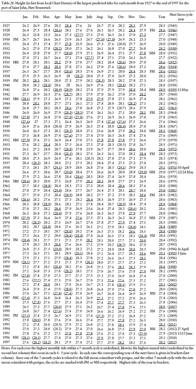
12.6. BOUNDARY ISSUES
386 In common law, private ownership of land ends at the mean high water mark, and title to the area between the MHW and low water marks (so-called tidelands) is held by the sovereign states. In a leading U.S. Federal case, the United States Supreme Court referred to: "the mean high tide line which is neither the spring tide nor the neap tide, but the mean of all the high tides." Unfortunately, in other cases a different line is used, for example the vegetation line, the highest winter tide, and the mean higher high tide; a few states use the low water line as boundary (Bostwick and Ketchum 1972). Quite apart from the choice of tidal cycle, this lack of standardization bedevils tidal boundary issues on national and international scales. A long-term cycle was taken into account in the U.S.A. in the so-called "Borax" decision (United Sates Supreme Court 1935). In this landmark case in 1935, the United States Supreme Court ruled that "an average 18.6 years of tidal observations should be used to determine the datum elevation". Promoted in the U.S.A., this has been described as a progressive decision which incorporates the most accurate methodology for determining tidal boundaries. However the definition does not deal with submergence of the landmass in relation to mean sea level, difficulties in areas with diurnal or strongly mixed diurnal and semidiurnal tides, and non-tidal influences. Furthermore the 18.6 year cycle is based on the period of revolution of the Moon's nodes and during this period the diurnal inequality of the tides varies in strength.
387 The 1949 "Tide and Current Glossary" prepared for the U.S. Coast and Geodetic Survey defines MHW as "the average height of the high water over a 19-year period". For shorter periods of observation, corrections are applied to eliminate known variations and reduce the result to the equivalent of a mean 19-year value. The 19-year cycle, the so-called "Metonic Cycle", was chosen because 235 lunations occur almost exactly in 19 mean solar years, and this is in step with the Julian calendar (Greulich 1979). Named for its discoverer, the Greek astronomer Meton (432 B.C.), this cycle was used by the Nicene Council in 325 A.D. to fix the date of Easter.
388 Unfortunately, in legal cases where tidal heights are important, the emphasis placed on cycles of 18.61 (and 19 years) may not be warranted. This is the case in regions like the Bay of Fundy where diurnal inequality of the tides is of such minor importance that it can be virtually ignored among variations caused by the coincidence of perigean and spring tides. Table 22 shows the situation with respect to long term cycles of conditions leading to stronger and weaker than normal tides. Note that if one used 246 anomalistic months (18.558 years), 247 anomalistic months (18.634 years), or 252 anomalistic months (19.011 years), the multiples of other types of months are not nearly as closely matched as with 18.03 years. Thus, the courts may easily be led astray by misapplying astronomical data.
389 In theory, the height reached at High Water is the full amplitude above MSL, which is defined as the level that oceanic water would assume if no tidal or atmospheric influences are acting upon it. On land, the datum used by geodesists, surveyors, and engineers, is the Geodetic Survey of Canada Datum (GSCD, or GD). This datum is based on the value of Mean Sea Level prior to 1910 as determined from a period of observations at tide stations at Halifax and Yarmouth, N.S., and Pointe au-Père, Québec, on the east coast, and Prince Rupert, Vancouver and Victoria, British Columbia, on the west coast. In 1922 this was adjusted in the Canadian levelling network. Because in most areas of the Maritime Provinces the landmass is submerging relative to MSL, geodetic datum drops gradually below Mean Sea Level. Thus, local MSL at present is about 280 mm (0.9 ft) higher than G.D. However, there is a dearth of data, and no one is certain what the exact difference is between GSCD and MWL at different stations. This situation is troublesome for engineers and biologists who need to know the proper relation between the two datums at particular places and it is no less likely to trouble legal minds.
12.7. DETERMINATION OF MHW, BAY OF FUNDY
390 A legal decision regarding tidal issues in the Bay of Fundy resulted from the 1962 to 1965 trial proceedings in the case of Irving Limited and the Municipality of the County of Saint John vs. Eastern Trust Company. This trial (for details see Desplanque and Mossman 1999a) highlighted a wholesale incorrect use of tidal data and definitions. Central to this case was the definition of Mean High Water (MHW). In brief, it transpires that no matter what is chosen as a MHW elevation, the value employed in the Irving case has no valid statistical basis.
391 In retrospect, it is instructive to consider the manner in which MHW (and HHW) vary according to the increased tidal range toward the head of the Bay of Fundy. This will be illustrated for the Minas Basin, where seven principal tidal constituents account for more than 90% of the total variability of the tides (see Table 3). Note that while the amplitudes of these semidiurnal tides increase toward the head of the Bay and Basin, the diurnal amplitudes remain virtually constant at 0.2 meters. The shallow-water tides are relatively small, but will certainly become large for locations within estuaries. No constituents are available for the tides within the estuaries. However the diurnal tides probably will not be altered when progressing into the estuaries. Semidiurnal amplitudes are clearly a function of the distance from the port of Saint John where the principal tidal hydrographic station is located. Thus as shown in section 5.3.2, the range of the dominant semidiurnal tides in the Bay of Fundy increases exponentially as they advance, at the rate of about 0.36% per kilometre. This allows local tidal range to be estimated very accurately, with reference to Geodetic Datum, from which follow realistic estimates of MWL and HHW.
392 The above relationship is, among other things, relevant to proposed tidal power schemes in the Bay of Fundy. These might very well modify the tidal regime (Greenberg 1987) and conceivably lead to international legal conflicts. Indeed a model used during the 1977 studies for Fundy tidal power development concluded that should a tidal power plant be built in the Minas Basin, the amplitude of average tides would increase by 0.15 m along the Gulf of Maine coastline of New England, and up to 0.25 m along New Brunswick coastline. Whatever the truth of this dire prediction, the fact is that coastal submergence is a reality that must be faced due to continuing sea-level rise. No protest, political or otherwise, can alter this situation. Further, if MHW is to be established, one has to make the choice between a permanent level linked to a certain year such as the Geodetic Datum of Canada, or a level which moves with changes in sea level due to geomorphological influences triggered by eustatic sea-level rise.
393 When the International Court of Justice set the boundary line between Canada and the United States through the Gulf of Maine, in October 1984, people on both sides of the border protested that the Court had decreased the area of the Gulf of Maine to such a degree that many jobs would be lost in both countries. If that same Court has to make a decision about changing characteristics of the tides and water levels in the Gulf of Maine-Bay of Fundy system, our knowledge of these characteristics had better be able to stand up to close examination.
12.8. THE BOTTOM LINE
394 An interdisciplinary approach is needed in the matter of tidal boundary delimitation. However, whatever the roles of lawyers, surveyors and scientists, the terms MHW and MLW need to be unambiguously defined in accordance with modern tidal and astronomical principles and terminology. European tidal conditions taken as standard in legal circles are not universal and consequently do not permit recognition of various common types of tides such as those governed by diurnal inequalities. Establishment of tidal boundaries is impossible when courts assume non-existent conditions.
395 Tidal datums are commonly misconceived to be fixed planar levels rather than undulating time and space-dependent surfaces. Yet, except for non-astronomical factors such as storm surges, tectonic activity and postglacial sea-level rise, tidal prediction with reference to specific tide levels can be made with a high degree of confidence. In fact there is a tendency to give greater credence to the predictions and the tidal constituents on which they are based than to the observed tides. However, if the procedure is correct, the average of the predicted and observed heights should be close together. The more accurate establishment of tidal datums hinges on improved prediction, which in turn requires more reference ports, updated tidal information and improved surveying techniques. Where numerous ports exist as along the eastern Canadian seaboard and the M2 tidal constituent is dominant, the amplitude of the M2 tide as measured above local MSL, closely approaches MHW. Also, the exponential increase in amplitude of the semidiurnal tides in the Bay of Fundy allows MWL, HHW and the local tidal ranges to be predicted quite accurately in this home to the world's highest tides.
13. Conclusions (TOP)
396 The hydrodynamic vigour of the Bay of Fundy rules over such geologically significant processes as erosion, sediment dynamics, and the Bay's natural resources and ecosystems. However, there is a clear need to more exactly evaluate the dynamics of the tidal regime in order to better understand the multitude of geological processes at work. Conclusions from investigations to date are summarized below.
- Along the eastern Canadian seaboard the M2 tidal constituent is dominant and the amplitude of the M2 tide as measured above MSL closely approaches MHW. MSL and MHW are rising in respect to the land at an average rate of 2 to 3 mm/year.
- As they advance toward the head of the Bay of Fundy, tidal ranges commonly exceed 15 m, and the amplitude of the dominant semidiurnal tides increases exponentially at the rate of 0.36 %/ km. This allows the local tidal range to be predicted very accurately, likewise MWL and HHW.
- An integral part of the western North Atlantic Ocean, the Bay of Fundy tides hydrodynamically exhibit the effects of a co-oscillating tide superimposed upon the direct astronomical tide.
- Forcing by the North Atlantic tide drives Bay of Fundy tides primarily by standing wave conditions developed through resonance; differences in the tidal range through the Bay of Fundy-Gulf of Maine-Georges Bank System are, in effect, governed by the rocking of a tremendous seiche.
- Although dominantly semidiurnal, Fundy tides nevertheless experience marked diurnal inequalities. The overlapping of the cycles of spring and perigean tides every 206 days results in an annual progression of 1.5 months in the periods of extra high tides.
- Extra-high tides can occur at all seasons in the Bay of Fundy, depending on the year in question. The result is considerable tidal variation throughout the year. Distinct cycles of 12.4 hours, 24.8 hours, 14.8 days, 206 days, 4.53 years, and 18.03 years are recognized.
- Three main astronomical tide-generating factors determine the number of tides that can exceed a certain elevation during any given year: the variable distance between the Earth and the Moon; the variable positions of the Moon, Sun, and Earth relative to each other; the declination of the Moon and Sun relative to the Earth's equator.
- Vigorous interplays between land and sea occur in northern macrotidal regimes. In Bay of Fundy estuaries, the rising sea level continually re-establishes salt marshes at higher levels despite infrequent floodings.
- The largest tides arrive in sets of 7 months, 4.53 years and 18.03 years, and most salt marshes are built up to the level of the average tide of the 18 year cycle. Assuming local marsh level to be 1.2 m beneath the high water level of extreme high tides, an empirical High Marsh Curve allows the number of annual floodings to be determined.
- Marigrams constructed for estuaries of rivers feeding into the Bay of Fundy show the tidal wave progressively reshaped over its course, and that its sediment-carrying and erosional capacities vary as a consequence of changing water surface gradients.
- Changing seasons effect substantial alterations in the character of estuaries. Thus winter contributes to an already complex tidal regime, especially during the second half of the 7-month cycle. Heaviest ice conditions occur one or two months before perigean and spring tides combine to form the largest tide of the cycle. At this time, the difference in height between neap tide and spring tide is increasing, resulting in the optimal time for flooding of marshlands.
- Changing environmental conditions in the Bay of Fundy may signal an increase in the dynamic energy of the tides. Observations indicate critical connections between tides, currents, erosion, sedimentation, and the biological community. There is a clear need to more precisely evaluate the dynamics of the tidal regime and to better understand the myriad geological processes at work.
Appendix: Glossary of Terms (TOP)
Aboiteau. Gated drainage sluice built into a dyke.
Amphidromic point. A point of zero amplitude of the observed or constituent tide.
Amphidromic system. A region surrounding an amphidromic point from which radiating cotidal lines progress through all hours of the tidal cycle.
Amplitude. Half the height or range of the wave, and the distance that the tide moves up or down from Mean Water Level.
Anomalistic cycle (monthly). Cycle in the average period (27.555 days) of the revolution of the Moon around Earth with respect to lunar perigee.
Aphelion. The point in Earth's orbit farthest from the Sun.
Apogean tide. Tide of decreased range occurring monthly when the Moon is in apogee.
Apogee. The point on the Moon's orbit that is farthest from Earth.
Argument. The angle indicated by the cosine term in an equation describing harmonic motion.
Astronomical tide (gravitational tide, equilibrium tide). The theoretical tide formed assuming that waters covering the face of the Earth instantly respond to the tide-producing forces of the Moon and Sun and form a surface of equilibrium under the action of these forces.
Barycentre. The combined centre of mass around which Earth and Moon revolve in essentially circular orbits.
CD. See "chart datum".
Celerity (of a wave). The speed or horizontal rate of advance of a wave.
Centrifugal force. Outward directed force acting on a body moving along a curved path or rotating about an axis.
Centripetal force. A centre-seeking force that tends to make rotating bodies move toward centre of rotation.
Chart datum (CD). An established elevation so low that the tides at that place will seldom if ever fall below it.
Constituents. The cosine terms in an equation describing tidal harmonic motion.
Continental shelf. Zone extending from the line of permanent immersion to the depth (average 130 m) where a steep descent occurs to great depths.
Coriolis effect. Also known as Coriolis force. An apparent force acting on a body in motion, due to rotation of the Earth causing deflection to the right in northern hemisphere and to the left in southern hemisphere.
Cotidal lines. Lines on a map giving the location of the tide's crest at stated time intervals.
Crest of a wave. Highest part of a propagating wave.
Current. A horizontal movement of water.
Declination. The angular distance of the Moon or Sun above or below the celestial equator.
Diurnal. Daily tides; having a period or cycle of approximately one tidal day.
Diurnal inequality. The difference in height between the two High Waters or the two Low Waters of each tidal day.
Drumlin. A streamlined hill of compact glacial fill formed by a glacier.
Dynamic tidal theory. Model of tides that takes into account the effects of finite ocean depth, basin resonances and the presence of continents.
Ecliptic. The plane of the centre of the Earth-Moon system as it orbits around the Sun; the intersection of the plane of Earth's orbit with the celestial sphere.
Equal High Water (EHW). Two daily high tides of equal height.
Equal Low Water (EHW). Two daily low tides of equal height.
Equilibrium theory. See "astronomical tide".
Equilibrium tide. Hypothetical tide due to the tide-producing forces under the equilibrium theory; also known as the gravitational tide.
Equinox. Times of the year when the Sun stands directly above the equator so that day and night are of equal length around the world (about 21 March and 22– 23 September).
Estuary. A coastal embayment into which fresh river water enters at its head and mixes with the relatively saline ocean water.
Eustatic. Pertaining to global changes of sea level that affected all oceans as a result of absolute changes in the quantity of sea water.
Evectional (monthly) cycle. The time required for the revolution of Moon around Earth, depending upon the variation of the eccentricity of its orbit.
Exponential (growth). A variable with a constant growth rate is said to increase exponentially.
Forced wave. A wave generated and maintained by a continuous force.
Free wave. A wave that continues to exist after the generating force has ceased acting.
Frequency of wave. The number of cycles that pass a location during a unit of time.
Gravity wave. A wave from which the restoring force is gravity.
Harmonic analysis. The mathematical process by which the observed tide or tidal current at any location is separated into harmonic constituents.
Head. The difference in water level at either end of a strait, channel, etc.
Height (range) of a wave. Vertical distance between wave crest and the adjacent wave troughs.
Higher High Water (HHW). The higher of two daily High Waters.
Higher High Water, large tide (HHWLT). Average of the highest high waters, one from each of 19 years of predictions.
Higher High Water, mean tide (HHWMT). Average of all the high waters from 19 years of predictions.
Higher Low Water (HLW). The higher of two daily Low Waters.
High Water (HW). Maximum height reached by a rising tide as a result of periodic tidal forces and the effects of meteorological, hydrologic and/or oceanographic conditions.
Holocene. The latest epoch of the Cenozoic era, from the end of the Pleistocene epoch to the present time. In northern latitudes, it generally equates with the postglacial interval.
Ice factories. Open water consisting of an unconsolidated mixture of needle-like ice crystals and sediment-laden waters.
Ice walls. Vertical walls of ice up to 5 m high formed in a rectangular estuarine channel under winter conditions.
Intertidal zone. The zone between mean higher high water and mean lower low water lines.
Isostatic compensation. Adjustment of crust of the Earth to maintain equilibrium among units of varying mass and density.
Julian calendar. Introduced by Julius Caesar 45 B.C.E., this calendar provided that the common year should consist of 365 days, and that every fourth year, now known as leap year, should contain 366 days, making the average length of the year 365.25 days. It differs from the modern (Gregorian) calendar in which the calendar century years not divisible by 400 are common years.
K 1. Luni solar diurnal constituent; with O1 it expresses the effect of the Moon's declination.
K 2. Luni solar semidiurnal constituent; it modulates amplitude and frequency of M 2 and S 2 for the declinational effect of the Moon and Sun, respectively.
Knot. Speed unit of one nautical mile (1852 metres) per hour.
L 2. Smaller lunar elliptic semidiurnal constituent; with N 2 it modulates the amplitude and frequency of M 2 for the effect of variation in the Moon's orbital speed due to its elliptical orbit.
Lag (deposit). Larger sedimentary particles remaining after smaller particles are washed away.
Latitude. Angular distance between point on the Earth and the equator measured north or south from the equator along a longitudinal meridian.
Longitude. Angular distance along the equator east and west of Greenwich measured in degrees or hours, the hour being taken as 15° of longitude.
Lower High Water (LHW). The lower of two daily High Waters.
Lower Low Water (LLW). The lower of two daily Low Waters, or a single Low Water.
Lower Low Water, large tide (LLWLT). Average of lowest low waters, one from each of 19 years of predictions.
Lower Low Water, mean tide (LLWMT). Average of all the lower low waters from 19 years of predictions.
Lowest Normal Tide (LNT). Currently synonymous with LLWLT; it is also called chart datum (CD).
Low Water (LW). Lowest height of the tide in daily cycle.
Lunar day. The time of Earth's rotation with respect to the Moon; mean lunar day = 24.84 solar hours.
Lunar month (synodical month). A period of 29 ½ days in which the Moon passes through four phases: new moon, first quarter, full moon, and last quarter.
M 1. Smaller lunar elliptic diurnal constituent; it helps to modulate the amplitude of the declinational K 1 for effect of the Moon's elliptical orbit.
M 2. Principal lunar semidiurnal constituent; it represents the rotation of Earth with respect to the Moon.
Macrotidal. Tidal system in which the tidal range exceeds 4 m.
Marigram (tidal curve). A graphical record of the rise and fall of the tide.
Mean Higher High Water (MHHW). The average of the Higher High Water height on all tidal days observed during a tidal datum epoch.
Mean High Water mark (MHW). The level reached by the M 2 amplitude above MSL; in Canada, usually taken as equivalent to "ordinary" high water (OHW).
Mean Low Water (MLW). The average of the Lower Low Water height of all tidal days during the tidal datum epoch.
Mean Lower Low Water (MLLW). The average of the Lower Low Water height on all tidal days observed during a tidal datum epoch.
Mean Sea Level (MSL). The level that oceanic water would assume if no tidal or atmospheric infl uences are acting upon it.
Mean Water Level (MWL). Average of all hourly water levels with respect to chart datum observed over the available period of record.
Meridian. Circle of longitude passing through the poles and any given point on Earth's surface.
Meterological tides. Tidal constituents having their origin in daily or seasonal variations in weather conditions which may occur with some degree of periodicity.
MHW. See Mean High Water mark.
Mixed tide. Tide having a conspicuous diurnal inequality in the Higher High and Lower High Waters and/or Higher Low and Lower Low Waters.
Moraine. Hill or ridge of sediment deposited by glaciers; geomorphologic name for a land form composed mainly of till deposited by either an extant or extinct glacier.
MSL. See Mean Sea Level.
MWL. See Mean Water Level.
N 2. Longer lunar elliptic semidiurnal constituent; with L 2 it modulates the amplitude and frequency of M 2 for the effect of variation in the Moon's orbital speed.
Neap tide. Tide occurring near the fi rst and last quarter of the moon, when the range of the tide is least.
Nodical month. Average period (27.212 days) of the revolution of the Moon around Earth relative to its passing through the ecliptic.
O 1. Lunar diurnal constituent; with K1 it expresses the effect of Moon's declination; and with P 1 it expresses the effect of the Sun's declination.
Ordinary High Water (OHW). In Canada, a level in surveying practice taken as equivalent to Mean High Water.
Outwash (glacial). Stratified detritus washed out from a glacier by melt water streams and deposited beyond the terminal moraine or margin of active glacier.
Overpressure. Excessive pressure.
Overtides. Analogous to overtones in music, and considered as higher harmonics of the fundamental tides.
P 1. Solar diurnal constituent; with K1 it expresses the effect of the Sun's declination.
Perigean tide. A spring tide occurring monthly when the Moon is at or near perigee of its orbit.
Perigee. The point on the Moon's orbit that is nearest Earth.
Perihelion. The point in Earth's orbit nearest to the Sun.
Period. Interval required for the completion of a recurring event or any specific duration of time.
Phase lag. Angular retardation of a maximum of a constituent of the observed tide behind the corresponding maximum of the same constituent of the equilibrium tide.
Prime meridian. Meridian of longitude passing through the original site of the Royal Observatory, Greenwich, England.
Progressive wave. A wave of moving energy in which the wave form moves in one direction along the surface of the medium.
Q 1. Larger lunar elliptic diurnal constituent; with (M 1), it modulates the amplitude and frequency of the declinational effects of the Moon and the Sun.
Refraction. The bending of the wave crest due to changing depths.
Resonance. Tidal motions on Earth are forced motions resulting in large scale oscillations analogous to a swinging bob of a pendulum. If the energy imparted exceeds the limits of true oscillation, a state of resonance is said to occur. If the dimensions of a gulf or sea allow for a period of free oscillation equal to that maintained in the ocean, resonance may occur.
S 2. Principal solar semidiurnal constituent; it represents this rotation of the Earth with respect to the Sun.
Salt marsh. A low-lying flat area of vegetated marine soils that is periodically inundated by saltwater.
Saros. The 18.03 yr cycle in which Moon, Sun and Earth return to almost identical relative positions; a cycle in which solar and lunar eclipses repeat themselves under approximately the same conditions.
Seiche. A standing wave oscillation of an enclosed or partly enclosed body of water that continues to oscillate after the generating force ceases.
Semidiurnal. Twice daily tides; having a period/cycle of approximately one-half of a tidal day.
Set up (of the wind). Flow of wind such that the water is driven toward the shore line.
Sidereal day. The time of Earth's rotation with respect to the vernal equinox.
Sidereal month. Average period (27.322 mean solar days) of the revolution of Moon around Earth relative to a fixed star.
Sidereal time. Time usually defined as the hour angle of the vernal equinox.
Sidereal year. Average period of the revolution of Earth around the Sun with respect to a fixed star.
Slack water. For a perfect progressive tidal wave, this occurs midway between high and low water.
Solar day. The period of Earth's rotation with respect to the Sun.
Solstice. Times of the year when the Sun stands above 23.5°N or 23.5°S latitude (about 22 December and 22 June).
Spring tide. Tide occurring near new and full moon, when the range of the tide is greatest.
Standard time. With few exceptions, standard time is based upon some meridian which differs by a multiple of 15° from the Greenwich meridian.
Standing wave. Type of wave in which the water surface oscillates vertically without progression between fixed nodes.
Storm surge. The local change in the elevation of the ocean along the shore due to a storm. It is measured by subtracting the astronomic tidal elevation from the total elevation.
Storm tide (storm surge). A sudden abnormal rise (positive) or fall (negative) of sea level due to change in atmospheric conditions along a coast. The sum of the storm surge and astronomic tide.
Synodical month. The average period of the revolution of the Moon around Earth relative to the Sun's position (29.531 days).
Thalweg. The median line of a stream or channel.
Tidal bore. A tidal wave that propagates up a relatively shallow and sloping estuary or river channel with a steep wave front, the leading edge rises abruptly, often with continuous breaking and commonly followed by several large undulations.
Tidal constituent (partial tide). A cosine curve representing the influence or characteristic of the local tide.
Tidal creek. Is a creek formed by tidal water that moves onto a tidal marsh during the Higher High Waters, discharging with the turn of the tide.
Tidal curve. See "marigram".
Tidal day. The time interval between two successive passes of the Moon over a meridian (about 24 hours, 50 minutes).
Tidal estuary. The mouth of a tidal river where the tidal flow regime shapes the channel bed.
Tidal prism. The top part of the estuary between the Low Water and the High Water levels.
Tidal range. Total vertical distance between High Water and Low Water. Note. In Canadian Tide Tables, the range at a given location is the distance between Higher High Water and Lower Low Water.
Tidal river. The stretch of a fresh water river where the dominant factor shaping the channel is fresh water.
Tide. The periodic rise and fall of a body of water resulting from gravitational interaction between Sun, Moon and Earth.
Tide producing force. That part of the gravitational attraction of the Moon and Sun which is effective in producing the tides on Earth.
Tide wave (tidal wave). Long period gravity wave originating in the tide-producing force and manifest in tidal ebb and flow.
Tiding (warping). Transformation of salt marsh into grasslands by use of canals to focus tidal inundations of sediment-charged seawater.
Tractive force. The horizontal component of a tide-producing force vector.
Tropical monthly cycle. The average period (about 27.322 days) of the evolution of the Moon around Earth relative to the vernal equinox.
Trough. The lowest point in a propagating wave.
Tsunami. A seismic sea wave; in literal translation from Japanese meaning "a long wave in harbour".
Universal time. Same as Greenwich Mean Time.
Vernal equinox. See "equinox".
Wave height. The vertical distance between crest and trough.
Wave length. Horizontal distance between two successive wave crests or troughs.
Wave train. A series of waves from the same direction; also known as a wave set.
Z 0. Symbol recommended by the International Hydrographic Organization to represent the elevation of mean sea level above chart datum.
Acknowledgements (TOP)
We are pleased to acknowledge that selected source materials for this work derived from the Maritime Marshlands Rehabilitation Administration (MMRA) observations (1950– 1965), and from Maritime Resource Management Services (MRMS) archives (1972– 1987), Amherst, Nova Scotia. This research has been facilitated by a grant in aid of research (#A8295) to DJM from the Natural Sciences and Engineering Research Council of Canada. We are likewise grateful to Mount Allison University for financial and logistical assistance. Helpful advice and friendly discussions have been generously contributed by individuals at the Bedford Institute of Oceanography, Dartmouth, Nova Scotia: J. Shaw, A.C. Grant, G. Fader, R.B. Taylor and D. Frobel of Geological Survey of Canada (Atlantic), Natural Resources Canada; and C.T. O'Reilly, B. Petrie and D. Greenberg of Fisheries and Oceans Canada. Special thanks to journal referees J. Shaw and C. Hannah for their important productive criticism. The advice of G.N. Ewing, former Dominion Hydrographer, on regional tides is greatly appreciated, likewise that of D.L. DeWolfe, formerly of the Canadian Hydrographic Service, on North Atlantic tides. P. Cant, Sackville, N.B. kindly provided valuable advice on extensive portions of an early draft of this paper. Early collaborations by the senior author with C.L. Amos (formerly of GSCA), D.C. Gordon (DFO) and D.I. Bray (University of New Brunswick) are freely acknowledged. D. Estabrooks and A. Estabrooks competently assisted with typing, formatting and layout. We are especially appreciative, too, of the extensive constructive editorial advice received from R.A. Fensome (Geological Survey of Canada, Atlantic) during the final pre-publication period. Reproduction of certain portions of our previously published material has been generously permitted by Geoscience Canada, Atlantic Geology and The Geographical Review, and for this we are grateful.References (TOP)
Abell, G.O., Morrison, D., & Wolff, S.C. 1988. Realm of the Universe. Saunders College Publishing, 529 p. (4 th edition)
Acres, H.G., & Company 1946. Report on Tidal Power, Petitcodiac and Memramcook estuaries, Province of New Brunswick, 1945. Canada: Department of Mines and Resources, Surveys and Engineering Branch – Dominion Water and Power Bureau, King's Printer, Ottawa, Ontario; two volumes, 75 p.
Allen, J.R.L. 1995. Salt-marsh growth and fluctuating sea level: implications of a simulation model for Flandrian coastal stratigraphy and peat-based sea-level curves. Sedimentary Geology, 100, pp. 21– 45.
ASCE (American Society of Civil Engineers) 1962. Nomenclature for hydraulics. American Society of Civil Engineers Manual and Report on Engineering Practice, no. 43, 501p.
Amirault, J.F., & Gates, A.D. 1976. The storm of 2 February, 1976, in the Maritime Provinces. Atmospheric Environmental Service, Scientific Series, Report no. MAES 7-76, 8 p.
Amos, C.L. 1978. The post-glacial evolution in the Minas Basin, Nova Scotia: a sedimentological interpretation. Journal of Sedimentary Petrology, 48, pp. 965– 982.
Amos, C.L. 1995a. The dynamics of siliciclastic tidal flats. In The Geomorphology and Sedimentology of Estuaries. Elsevier, Amsterdam, The Netherlands, pp. 1– 55.
Amos, C.L. 1995b. Siliciclastic tidal flats. In Developments in Sedimentology, No. 53. Edited by G.M.E. Perillo. Elsevier, Amsterdam, The Netherlands, pp. 273– 306.
Amos, C.L., & Joice, G.H.E. 1977. The sediment budget of the Minas Basin, Bay of Fundy, N.S. Bedford Institute of Oceanography, Data Series/BI-D-77-3/June 1977, 410p.
Amos, C.L., & Tee, K.T. 1989. Suspended sediment transport processes in Cumberland Basin, Bay of Fundy. Journal of Geophysical Research, 94, pp. 1407– 1417.
Amos, C.L., Tee, K.T., & Zaitlin, B.A. 1991. The post-glacial evolution of Chignecto Bay, Bay of Fundy, and its modern environment of deposition. In Clastic Tidal Sedimentology. Edited by D.G. Smith, G.E. Reinson, B.A. Zaitlin and R.A. Rahmani. Canadian Society of Petroleum Geologists, Memoir 16, pp. 59– 89. (1 st edition)
Apel, J.R. 1987. Principles of Ocean Physics. Academic Press, New York, New York, 634 p.
Apollonio, S. 1979. The Gulf of Maine. Courier-Gazette, Rockland, Maine, 36 p.
Atlantic Tidal Power Programming Board. 1969. Appendix 3. In Feasibility of Tidal Power Development in the Bay of Fundy. Governments of Canada, New Brunswick and Nova Scotia. Atlantic Tidal Power Programming Board, Halifax, Nova Scotia, 38 p.
Baird, W.W. 1954. Report on Dykeland Reclamation 1913 to 1952. Canadian Department of Agriculture, Experimental Farms Service, Ottawa, Ontario, 63 p.
Baker, G.C. 1982. Some historical aspects of tidal power. In New Approaches to Tidal Power, June 1, 1982, Dalhousie University, Halifax, Nova Scotia, 9 p.
Bartsch-Winkler, S., & Lynch, D.K. 1988. Catalog of worldwide tidal bore occurrences and characteristics. United States Geological Survey, Circular 1022, 17 p.
Bay of Fundy Tidal Power Review Board. 1977. Reassessment of Fundy tidal power. Reports of the Bay of Fundy Tidal Review Board and Management Committee. Canada Ministry of Supply and Services, Ottawa, Ontario, 516 p.
Bleakney, J.S.B. 1986. A sea-level scenario for Minas Basin. In Effects of changes in sea level and tidal range on the Gulf of Maine – Bay of Fundy system. Edited by G.R. Daborn. Acadia Centre for Estuarine Research, Publication no. 1, pp. 123– 125.
Bostwick, J., & Ketchum, B.H. 1972. The Water's Edge: Critical Problems of the Coastal Zone. MIT Press, Cambridge, Massachusetts.
Bray, D.I., Demerchant, D.P., & Sullivan, D.L. 1982. Some hydrotechnical problems related to the construction of a causeway in the estuary of the Petitcodiac River, New Brunswick. Canadian Journal of Civil Engineering, 9, pp. 296– 307.
Cabilio, P., Dewolfe, D.L., & Daborn, G.R. 1997. Fish catches and long-term tidal cycles in Northwest Atlantic fisheries: a nonlinear regression approach. Canadian Journal of Fisheries and Aquatic Science, 44, pp. 1890– 1897.
Canadian Hydrographic Service. 1964. Canadian Tide and Current Tables 1: Atlantic Coast and Bay of Fundy. Department of the Environment, Ottawa, Ontario, 259 p.
Canadian Hydrographic Service. 1969a. Bathymetric Chart, Bay of Fundy to Gulf of St. Lawrence. Charts # 801 and # 802. Department of the Environment, Ottawa, Ontario.
Canadian Hydrographic Service. 1969b. Harmonic Constants and Associated Data for Canadian Waters. 1: Atlantic Coast (Non-paginated collection of data). Department of the Environment, Ottawa, Ontario.
Canadian Hydrographic Service. 1973. Canadian Tide and Current Tables, Volumes 1, 2, and 3. Marine Science Directorate, Department of the Environment, Ottawa, Ontario.
Canadian Hydrographic Service. 1979. Hydrographic Chart D-4003. Department of the Environment, Ottawa, Ontario.
Canadian Hydrographic Service. 1981. List of Tidal Constituents of 60 ports along the eastern seaboard from Newfoundland to Cape Cod. (Miscellaneous data). Department of the Environment, Ottawa, Ontario.
Canadian Tide and Current Tables. 2004. Atlantic Coast and Bay of Fundy, Volume 1. Fisheries & Oceans Canada, Ottawa, Canada, 89 p.
Carter, R.W.G. 1998. Coastal Environments. Academic Press, Harcourt Brace, London, U.K., 617 p. (4 th printing)
Chalmers, R. 1895. Report on the surface geology of eastern New Brunswick, northwestern Nova Scotia, and of a portion of Prince Edward Island. Geological Survey of Canada, Annual Report 1894, v. 7, part M, 135 p.
Charlier, R.H. 1982. Tidal Energy. Van Nostrand, New York, New York, 351 p.
Clancy, E.P. 1969. The Tides: Pulse of the Earth. Anchor Books. Doubleday, New York, New York, 228 p.
Conkling, P.W. (Editor). 1995. From Cape Cod to the Bay of Fundy - an Environmental Atlas of the Gulf of Maine. MIT Press, Cambridge, Massachusetts, 258 p.
Daborn, G.R. (Editor). 1977. Fundy tidal power and the environment. Proceedings of Workshop held at Acadia University, Acadia University Institute, Wolfville, Nova Scotia, 304 p.
Daborn, G.R., & Dadswell, M.J. 1988. Natural and anthropogenic changes in the Bay of Fundy-Gulf of Main-Georges Bank system. In Natural and Man-Made Hazards. Edited by: M.I. El-Sabh and T.S. Murty. D. Reidel Publishing, Dordrecht, The Netherlands, pp. 547– 560. (1 st edition)
Dai Zeheng. 1982. Reclaiming against the Qiantang Bore. Zhejiang Provincial Institute of Estuarine and Coastal Engineering Research, Hangzhou, China, 13 p.
Darwin, G.H. 1898. The Tides and Kindred Phenomena in the Solar System. John Murray, London, United Kingdom, 369 p.
Davis, D.S. 1943. Empirical Equations and Nomography. McGraw-Hill, New York, New York, 200 p.
Davis, D.S., & Browne, S.S. (Editors). 1996. The Natural History of Nova Scotia – Topics and Habitats. Nova Scotia Museum of Natural History and Nimbus Publishing, Halifax, Nova Scotia, 517 p. (3 rd edition)
Dawson, W.B. 1920. Tides at the head of the Bay of Fundy. Department of Naval Service, Ottawa, Ontario, 34 p.
Defant, A. 1958. Ebb and Flow. University of Michigan Press, Ann Arbour, Michigan.
Defant, A. 1961. Physical Oceanography. Pergamon Press, New York, New York, v. 1, 727 p., v. 2, 598 p.
Dekker, A.G., & Van Huissteden, J. 1982. Report of a geological investigation of the Tantramar marshes. Unpublished Report, Free University, Amsterdam 56 p. + 18 profiles.
Desplanque, C. 1952. De dykelands in de Maritime Provinces van Canada. Tijdschrift van de Nederlandse Heidemaatschappij, 63, pp. 14– 20.
Desplanque, C. 1974. The Saros and the Saxby Tide. Unpublished document C.D.74.1.21. Maritime Resource Management Service, Amherst, Nova Scotia, 12 p.
Desplanque, C. 1977. What is meant by High Water mark? Internal Report, Maritime Resource Management Service of Council of Maritime Provinces, 8 p.
Desplanque, C. 1980. The tides in the Bras d'Or Lake system. In Barra Strait Crossing, Cape Breton, Nova Scotia. Unpublished report prepared for Nova Scotia Department of Transportation (Maritime Resource Management Service, Amherst, Nova Scotia), 48 p.
Desplanque, C. 1985. Observations on the ecological importance of salt marshes in the Cumberland Basin, a macrotidal estuary in the Bay of Fundy. Estuarine, Coastal and Shelf Science, 20, pp. 205– 227.
Desplanque, C., & Bray, D.I. 1986. Winter ice regime in the tidal estuaries of the northeastern portion of the Bay of Fundy, New Brunswick. Canadian Journal of Civil Engineering, 13, pp. 130– 139.
Desplanque, C., & Mossman, D.J. 1998a. Tides and Coastal Processes in the Bay of Fundy. Unpublished report, Mount Allison University, Sackville, New Brunswick, 339 p.
Desplanque, C., & Mossman, D.J. 1998b. A review of ice and tide observations in the Bay of Fundy. Atlantic Geology, 34, pp. 195– 209.
Desplanque, C., & Mossman, D.J. 1999a. The water's edge: resolving tidal boundary problems in the coastal zone. In Proceedings of the Canadian Coastal Conference, Victoria, British Columbia, May 19– 22, 1999, Volume 1, pp. 77– 98.
Desplanque, C., & Mossman, D.J. 1999b. Storm tides of the Fundy. The Geographical Review, 89, pp. 23– 33.
Desplanque, C., & Mossman, D.J. 2001a. Fundamentals of Fundy tides. In Opportunities for protecting, restoring and enhancing coastal habitats in the Bay of Fundy; Proceedings of the 4 th Bay of Fundy Science Workshop, Saint John, New Brunswick, Sept. 19– 21, 2000. Edited by T. Chopin and P.B. Wells. Environment Canada, Atlantic Region Occasional Report, no. 17, pp. 178– 204.
Desplanque, C., & Mossman, D.J. 2001b. Bay of Fundy tides. Geoscience Canada, 28, (1), pp. 1– 11.
Dewolfe, D.L. 1981. Atlas of Tidal Currents – Bay of Fundy and Gulf of Maine. Canadian Hydrographic Service, Ottawa, 36 p.
Dionne, J.C. 1989. An estimate of shore ice action in a Spartina tidal marsh, St Lawrence Estuary, Quebec, Canada. Journal of Coastal Research 5, (2), pp. 281– 293.
Doodson, A.T., & Warburg, H.D. 1941. Admiralty Manual of Tides. His Majesty's Stationary Office, London, U.K., 270 p.
Dunn, B. 1985. The Acadians of Minas. National Historic Parks Branch, Parks Canada; Environment Canada, Ottawa, Ontario, 30 p.
Eagleson, P.S., & Dean, R.G. 1966. Small amplitude wave theory. In Estuary and Coastline Hydrodynamics. Edited by A.I. Ippen. McGraw-Hill, New York, New York, pp. 1– 77.
Fader, G.B.J. 1989. A late Pleistocene low sea-level stand of the southeast Canadian offshore. In Late Quaternary Sea-Level Correlation and Applications. Edited by D.B. Scott, P.A. Pirazolli and C.H. Honig. Kluwer Academic Publishers, Dordrecht, The Netherlands, pp. 71– 103.
Fader, G.B.J. 1996. Chapter 2. Aggregate assessment and sediment transport. In The Physical Environment of the Bay of Fundy – Fundy Issues Workshop, Wolfville, Nova Scotia, January 29, 1996. Edited by J.A. Percy, P.G. Wells and A Evans.
Fader, G.B.J., King, L.H., & MacLean, B. 1977. Surficial geology of the eastern Gulf of Maine and Bay of Fundy. Canadian Hydrographic Services, Marine Science Paper 19; and Geological Survey of Canada Paper 76-17, 23 p.
Fairbridge, R.W. 1966. The encyclopaedia of oceanography. Encyclopaedia of Earth Sciences Series, v.1. Dowden, Hutchinson & Ross, Stroudsburg, Pennsylvania, 1021 p.
Fairbridge, R.W. 1987. The spectra of sea level in a Holocene time frame. In Climate: History, Periodicity and Predictability. Edited by M.R. Rampiro, J.E. Saunders, W.S. Newman and L.K. Konigsson. Van Nostrand Reinhold, New York, New York, pp. 127– 142.
Falcon-Lang, H.J., Fensome, R.A., & Venugopal, D.V. 2003. The Cretaceous age of the Vinegar Hill silica sand deposit, southern New Brunswick: evidence from palynology and aleobotany. Atlantic Geology, 39, pp. 39– 46.
Forrester, W.D. 1983. Canadian Tidal Manual. Canadian Hydrographic Service, Department of Fisheries and Oceans, Ottawa, Ontario, 138 p.
Ganong, W.F. 1911. A preliminary study of Saxby Gale. Bulletin of the Natural Historical Society of New Brunswick, no. XXIXX. v. VI, Part III, p. 325– 339.
Garrett, C. 1970. Tidal resonance in the Bay of Fundy and Gulf of Maine. Nature, 238, pp. 441– 443.
Gehrels, W.R., Belknap, D.F., Pearce, B.R., & Gong, B. 1995. Modelling the contribution of the M2 tidal amplification to the Holocene rise of mean high water in the Gulf of Maine and the Bay of Fundy. Marine Geology, 124, pp. 71– 85.
Godin, G. 1990. Theory of exploitation of tidal energy and its application to the Bay of Fundy. Journal of the Fisheries Research Board, Canada, 26, pp. 2887– 2957.
Godin, G. 1992. Possibility of rapid changes in the tide of the Bay of Fundy, based on a scrutiny of the records from Saint John. Continental Shelf Research, 12, pp. 327– 338.
Gordon, D.C. 1984. Integration of ecological and engineering aspects in planning large scale tidal power development in the Bay of Fundy, Canada. Water Science Technology, 16, pp. 281– 295.
Gordon, D.C. Jr., & Dadswell, M.J. 1984. Update on marine environmental consequences of tidal power development in the upper reaches of the Bay of Fundy. Canada Technical Report on Fisheries and Aquatic Science, no. 1256, 686 p.
Gordon, D.C., & Desplanque, C. 1981. Ice dynamics in the Chignecto Bay region of the Bay of Fundy. Proceedings of the Workshop on Ice Action on Shores, Rimouski, Quebec; sponsored by the Associate Committee for Research on Shoreline Erosion and Sedimentation. National Research Council of Canada, Ottawa, Ontario, pp. 35– 52.
Gordon, D.C., & Desplanque, C. 1983. Dynamics and environmental effects of ice in the Cumberland Basin of the Bay of Fundy. Canadian Journal of Fisheries and Aquatic Sciences 40, pp. 1331– 1342.
Gordon, D.C., Crawford, D.J., & Desplanque, C. 1985. Observations on the ecological importance of salt marshes in the Cumberland Basin, a macrotidal estuary in the Bay of Fundy. Estuarine, Coastal and Shelf Science, 20, pp. 205– 227.
Grant, D.R. 1970. Recent coastal submergence of the Maritime Provinces, Canada. The Canadian Journal of Earth Sciences, 7, pp. 676– 689.
Grant, D.R. 1975. Recent coastal submergence of the Maritime Provinces. Proceedings of the Nova Scotia Institute of Science, 27, supplement 3, pp. 83– 107.
Grant, D.R. 1985. Glaciers, sediment and sea level, northern Bay of Fundy, Nova Scotia. 14 th Arctic Workshop; Arctic Land-Sea Interaction; Field Trip B, November 6– 8, 36 p.
Grant, D.R. 1989. Quaternary geology of the Atlantic Appalachian region of Canada. In Geology of Canada, No. 1, Geology Survey of Canada, Edited by R. J. Fulton, pp. 393– 440 (also Geological Society of America, The Geology of North America, v. K-1).
Greenberg, D.A. 1979. A numerical model investigation of tidal phenomena in the Bay of Fundy and Gulf of Maine. Marine Geodesy, 2, pp. 161– 187.
Greenberg, D.A. 1987. Modelling tidal power. Scientific American, 257 (1), pp. 128– 131.
Greenberg, D.A., Petrie, B.D., Daborn, G.R., & Fader, G.B. 1996. The physical environment of the Bay of Fundy. In Bay of Fundy Issues: a scientific overview; Workshop Proceedings, Wolfville, Nova Scotia, January 29 to February 1, 1996. Edited by J.A. Percy, P.G. Wells and A.J. Evans. Environment Canada, Atlantic Region Occasional Report no. 8, pp. 11– 34.
Greenough, J.D. 1995. Chapter 6. Mesozoic rocks. In Geology of the Appalachian - Caledonian Orogen in Canada and Greenland. Edited by H. Williams, Geological Survey of Canada, Geology of Canada, no. 6, pp. 567– 600 (also Geological Society of America, The Geology of North America, v. F-1.
Greulich, G.H. 1979. Definition of Mean High Water Line. Technical Notes. Journal of the Surveying and Mapping Division; Proceedings of the American Society of Civil Engineers, 105: No. SU1. Nov. 1979, pp. 111– 113.
Griffiths, N.E.S. 1992. The Contexts of Acadian History 1686 – 1784. McGill - Queens University Press, Montreal, Quebec, 137 p.
Hale, M. 1667. De jure maris: as reported in Attorney-General vs. Chambers (1854) 4 Deg. M and G 206, 43 ER. 486, p. 487.
Hansen, P.L. 1970. Hydraulic model study of the Reversing Falls at Saint John, New Brunswick. M. Eng. Thesis, Department of Civil Engineering, University of New Brunswick, 116 p.
Harvey, J., Coon, D., & Abouchar, J. 1998. Habitat Lost: Taking the Pulse of Estuaries in the Canadian Gulf of Maine. Conservation Council of New Brunswick, Fredericton, New Brunswick, 81 p.
Hicklin, P.W., Linkletter, L.E., & Peer, D.L. 1980. Distribution and abundance of Corophium volutator (Pallas), Macoma balthica (L.) and Heteromastus fi liformis (Claparéde) in the intertidal zone of Cumberland Basin and Shepody Bay, Bay of Fundy. Canadian Technical Report of Fisheries and Aquatic Sciences, no. 965, pp. 69– 77.
Hicks, B.C. 1965. Fundy tidal power. Electrical News and Engineering, October 1965, p. 46– 49.
Hill, J., Hill, P., Carrière, C., & Frobel, D. 1996. The Recent Ice Age. Video Guide. Atlantic Geoscience Society, Special Publication 13, 108 p.
Hind, H.Y. 1875. The ice phenomena and tides of the Bay of Fundy, considered in connection with the construction of the Baie Verte canal. The Canadian Monthly and National Review, 8 (3), pp. 189– 203.
Historia Naturalis, 1962. Pliny, the Elder; translated by Philemon Holland, Centaur Press, London, U.K., 496 p.
House, M.R. 1995. Orbital forcing time scales: an introduction. In Orbital Forcing Time Scales and Cyclostratigraphy. Edited by M.R. House and A.S. Gale, Geological Society Special Publication, no. 85, pp. 1– 18.
Jarrett, J.T. 1976. Tidal prism-inlet area relationships. Technical Report 3, General Investigation of Tidal Inlets, United States Army Coastal Engineering Research Centre, Fort Belvoir, Virginia, 12 p.
Jennings, S.C., Carter, R.W.G., & Orford, J.D. 1993. Late Holocene salt marsh development under a region relative-sea-level rise; Chezzetcook Inlet, Nova Scotia: implications for the interpretation of palaeomarsh sequences. Canadian Journal of Earth Sciences, 30, pp. 1374– 1384.
Johnson, D. 1925. The New England-Acadian Shoreline. Hafner, New York, New York, 609 p.
Keen, M.J., & Piper, D.J.W. 1990. Chapter 1. Geological and historical perspective. In Geology of the Continental Margin of Eastern Canada. Edited by M.J. Keen & G.L. Williams, Geological Survey of Canada, no. 2, pp. 5– 30 (also Geological Society of America, The Geology of North America v. I-1).
Keppie, J.D. 1982. The Minas Geofracture. In Major Structural Zones and Faults of the Northern Appalachians. Edited by P. St. Julien and J. Beland. Geological Association of Canada, Special Paper 24, pp. 1– 34.
Kerr, L.C. 1977. Coastal Law. Internal Report of Land Registration and Information Service of the Council of Maritime Provinces, 39 p.
Ketchum, B.H. (Editor). 1972. The water's edge: critical problems of the coastal zone. Proceedings of Coastal Zone Workshop, 22 nd May– 3rd June, 1972, Institute of Ecology and Woods Hole Oceanographic Institution, Woods Hole, Massachusetts, 393 p.
King, L.H., & MacLean, B. 1976. Geology of the Scotian Shelf. Geological Survey of Canada, Paper 74-31, 31 p.
Kjerfve, B. (Editor). 1988. Hydrodynamics of Estuaries. CRC Press Inc; Boca Raton, Florida, volume 1, 163 p. and volume 2, 125 p.
Knight, R.J., & Dalrymple, R.W. 1976. Winter conditions in a macrotidal environment, Cobequid Bay, Nova Scotia. In Le Glaciel, La Revue de Géographie de Montreal. Edited by J-C. Dionne, 30, pp. 5– 85.
Kwong, S.C.M., Davies, A.M., & Flather, R.A. 1997. A three-dimensional model of the principal tides on the European shelf. Progressive Oceanography, 39, pp. 205– 262.
La Forest, G.V. 1972. Water Law in Canada: The Atlantic Provinces. Information Canada, Ottawa, Ontario, 149 p.
Lambeck, K., Johnston, P., & Nakada, M. 1990. Holocene glacial rebound and sea level change in northwestern Europe. International Journal of Geophysics, 103, pp. 451– 468.
Lammers, W., & De Haan, F.A. 1980. De Holocene afzettingen in het gebied van de Tantramar en Aulac. (The Holocene deposits in the area of Tantramar and Aulac rivers). Report of Doctoral Fieldwork, Free University, Amsterdam, The Netherlands, 74 p + 18 profiles.
Larsen, P.F., & Topinka, J.A. (Editors). 1984. Fundy Tidal Power Development – Preliminary Evaluation of its Environmental Consequences to Maine. Report to the Maine State planning Office by Bigelow Laboratory of Ocean Sciences, 136 p.
Lauff, G.H. 1967. Estuaries. American Association for the Advancement of Science Publication no. 83, 757 p.
LeBlond, P.H., & Mysak, L.A. 1978. Waves in the Ocean. Elsevier, Amsterdam, The Netherlands.
Lorentz, H.A. 1926. Verslag Staatscommissie Zuiderzee. 1918– 1926. Algemeene Landsdrukkerij. The Netherlands. 345 p.
Lynch, D.K. 1982. Tidal Bores. Scientific American v. 246 (4), p. 146– 157.
MacLean, P. 1979. The Saxby gale. The Atlantic Advocate, January, 1979, p. 44– 47.
Maritime Marshland Rehabilitation Administration (MMRA) 1950– 1965. Annual Reports on Activities under the MMRA Act. Canadian Department of Agriculture, Ottawa, Ontario.
Masefield, J. 1924. The Travels of Marco Polo, the Venetian, with an introduction by John Masefield. J.M. Dent and Sons, London, U.K., 461 p. (Reprint of the 1854 edition, edited by Thomas Wright)
McIntyre, L. 1972. The Amazon: mightiest of rivers. National Geographic Magazine, 142, pp. 445– 495.
Milligan, D.C. 1987. Maritime Dykelands: the 350 Year Struggle. Nova Scotia Department of Government Services, Publishing Division, 110 p.
Montbarbut, J. 1985. Les Colon de l'Aunis et de la Saintonge au Canada, Regime français 1608– 1763. Association France-Canada-Brouage; l'Imprimerie Graphique de l'Ouest, 223 p.
Morrill, R.A., Chin, E.H., & Richardson, W.S. 1979. Maine coastal storm and flood of February 2, 1976. United States Geological Survey, Professional Paper, 1087, 20 p.
Mossman, D.J., & Grantham, R.G. 1996. The continental Jurassic of the Maritime Provinces, Canada. In The Continental Jurassic. Edited by M. Morales; Museum of Northern Arizona, Bulletin 60, pp. 427– 436.
NATO (Advanced Study Institutes Program). 1987. Quaternary glaciations, geomorphology, and sea-level changes: Bay of Fundy region. International Advanced Course (in co-operation with IGCP Project 200) on "Late Quaternary sea-level correlation and applications," July 20– 26. Centre for Marine Geology, Dalhousie University, Halifax, Canada. (Published by NATO)
Nichols, S.E. 1983. Tidal Boundary Delimitation. Department of Surveying and Engineering, University of New Brunswick, Technical Report no. 103, 202 p.
Noordijk, A., & Pronk, T. 1981. De Holocene afzettingen in de dalen van de Missaguash, LaPlanche and Nappan rivieren. Doctoral Scriptie, Free University, Amsterdam, The Netherlands, 64 p. + profiles.
Olsen, P.E., Schlische, R.W., & Gore, P.J.W. (Editors). Tectonic, depositional and paleontological history of early Mesozoic rift basins, eastern North America. Field Trip Guidebook, no T351; American Union, Washington, D.C., 174 p.
OPEN (The Open University Oceanic Course Team). 1993. Waves, Tides and Shallow-Water Processes. Open University and Pergamon Press, Oxford, U.K. 187 p.
Parkes, G.S., Ketch, L.A., & O'Reilly, C.T.O. 1997. Storm surge events in the Maritimes. Proceedings of Canadian Coastal Conference 1997, 21– 24 May, University of Guelph, Ontario, pp. 115– 129.
Pelletier, B.R. 1974. Sedimentary textures and relative entropy and their relationship to the hydrodynamic environment Bay of Fundy system. In Offshore Geology of Eastern Canada. Geological Survey of Canada, Paper 74-30, pp. 77– 94.
Peltier, W.R. 1999. Global sea level rise and glacial isostatic adjustment. Global and Planetary Change, 20, pp. 93– 123.
Percy, J.A., Wells, P.G., & Evans, A.J. (Editors). 1996. Bay of Fundy issues: a scientific overview; workshop proceedings, Wolfville, Nova Scotia. Environment Canada, Atlantic Region, Occasional Report No. 8, 191 p.
Pethick, J.S. 1984. An Introduction to Coastal Geomorphology. Arnold, London, U.K., 260 p.
Petrie, B. 1999. Sea level variability in the Bras d'Or Lakes. Atmosphere-Ocean, 37, pp. 221– 239.
Pilkey, O.H., Morton, R.A., Kelley, J.T., & Penland, S. 1989. Coastal Land Loss. Short Course in Geology: Volume 2. 28 th International Geological Congress. American Geophysical Union, Washington, D.C., pp. 9– 18. Pogany, G. 1958. Development of the Chignecto region. Moncton Daily Times, 13 June, 1958, p. 13.
Pomeroy, L.R., & Weigert, R.G. (Editors). 1981. The Ecology of a Salt Marsh. Springer-Verlag, Berlin, Germany, 271 p.
Postma, H. 1967. Sediment transport and sedimentation in the estuarine environment. In Estuaries. Edited by G.H. Lauff. American Association for the Advancement of Science, Publication 83, pp. 158– 179.
Pugh, D.T. 1987. Tides, Surges and Mean Sea-Level: a Handbook for Engineers and Scientists. J. Wiley & Sons, Chichester, U.K., 472 p.
Railsback, L.B. 1991. A model for teaching the dynamical theory of tides. Journal of Geological Education, 39, pp. 15– 18.
Rampino, M.R., Sanders, J.E., Newman, W.S., & Koenigsson, L.K. (Editors). 1987. Climate, History, Periodicity, and Predictability. Van Nostrand Reinhold Company, New York, New York, 588 p.
Ramsay, A. 1963. The composition of the submerged forest at Fort Lawrence, Nova Scotia. B.Sc. Honours. Thesis, Mount Allison University, 32 p.
Rao, D.B. 1968. Natural oscillations of the Bay of Fundy. Journal of Fisheries Research Board, Canada, 25, pp. 1097– 1114.
Raymond, W.O. 1910. The River Saint John – Its Physical Features. Legends and History from 1604 to 1784. Tribune Press, Saint John, New Brunswick, 552 p. (2 nd edition)
Redfield, A.C. 1980. Introduction to Tides. Marine Science International, Woods Hole, Massachusetts, 108 p.
Saxby, S.M. 1868. Coming weather. To the editor. Standard of London, 25 December, 1868 (no. 13 851, p. 5, column 7).
Schneider, D. 1997. The Rising Sea. Scientific American, 276 (3), pp. 112– 117.
Schott, C. 1955. Die Kanadischen Marschen. Universität Kiel, Geographische Institüt, Schriften, 15 (2), 59 p.
Schureman, P. 1941. A manual for the harmonic analysis and prediction of tides. United States Coast and Geodetic Survey, Special Publication no. 98, 416, 317 p.
Schureman, P. 1949. Tide and current glossary. United States Department of Commerce, Coast and Geodetic Survey, Special Publication no. 228, 40 p.
Schwiderski, E.W. 1980. On charting global ocean tides. Reviews in Geophysics and Space Physics, 18 (1), pp. 243– 268.
Scott, D.B. 1980. Morphological changes in an estuary: a historical and stratigraphical comparison. In The Coastline of Canada. Edited by S.B. McCann; Geological Survey of Canada Paper 80-10, pp. 199– 205.
Scott, D.B., & Collins, E.S. 1996. Late mid-Holocene sea-level oscillation: a possible cause. Quaternary Reviews, 15, pp. 851– 856.
Scott, D.B., & Greenberg, D.A. 1983. Relative sea-level rise and tidal development in the Fundy tidal system. Canadian Journal of Earth Sciences, 20, pp. 1554– 1564.
Scott, D.B., & Medioli, F.S. 1979. Marine emergence and submergence in the Maritimes. Unpublished Progress Report, Department of Energy Mines and Resources Research Agreement 45-4-79, 69 p.
Scott, D.B., & Medioli, F.S. 1986. Foraminifera as sea-level indicators. In Sea Level Research: a Manual for the Collection and Evaluation of Data. Edited by O. van de Plassche, Geo Books, Norwich, U.K., pp. 435– 455.
Scott, D.B., & Stea, R.R. 2000. Late Quaternary relative sea-level variations in the North Atlantic: comparison of mid-Holocene highstands to the last interglacial (isotopic stage 5e) highstands. Atlantic Geoscience Society Colloquium and Annual General Meeting, February 10– 12, Fredericton, New Brunswick, Program and Abstracts, p. 41.
Scott, D.B., Boyd, R., & Medioli, F.S. 1987. Relative sea level changes in Atlantic Canada: observed level and sedimentological changes vs theoretical models. In Sea Level Fluctuation and Coastal Evolution. Edited by D. Nummendal, O.H. Pilkey and J.D. Howard. Society of Economic Paleontologists and Mineralogists, Special Publication 41, pp. 87– 96.
Shaw, J., & Ceman, J. 1999. Salt-marsh aggradation in response to late-Holocene sea-level rise at Amherst Point, Nova Scotia, Canada. The Holocene, 9, pp. 439– 450.
Shaw, J., & Forbes, D.L. 1990. Short and long-term relative sea-level trends in Atlantic Canada. Proceedings, Canadian Coastal Conference 1990, Kingston, Ontario. National Research Council, Ottawa, Ontario, pp. 291– 305.
Shaw, J., Taylor, R.B., & Forbes, D.L. 1993. Impact of the Holocene transgression on the Atlantic coastline of Nova Scotia. Géographie physique et Quaternaire, 47, pp. 221– 238.
Shaw, J., Taylor, R.B., Forbes, D.L., Ruz, M-H., & Solomon, S. 1994. Sensitivity of the Canadian coast to sea-level rise. Geological Survey of Canada Open File Report, no. 2825, 114 p.
Shaw, J., Gareau, P., & Courtney, R.C. 2002. Palaeogeography of Atlantic Canada 13 – 0 kyr. Quaternary Science Reviews, 21, p. 1861– 1878.
Shepherd, P.C.F., Partridge, V.A., & Hicklin, P.W. 1995. Changes in sediment types and invertebrate fauna in the intertidal mudflats of the Bay of Fundy between 1977 and 1994. Canadian Wildlife Service, Technical Report Series, no. 237, 164 p.
Stea, R.R., & Pullan, S.E. 2001. Hidden Cretaceous basins in Nova Scotia. Canadian Journal of Earth Sciences, 38, pp. 1335– 1354.
Stea, R.R., Boyd, R., Fader, G.B.J., Courtney, R.C., Scott, D.B., & Pecore, S.S. 1994. Morphology and seismic stratigraphy of the inner continental shelf off Nova Scotia, Canada: evidence for a – 65 m lowstand between 11,650 and 11,250 C14 yr B.P. Marine Geology, 117, pp. 135– 154.
Stea, R.R., Piper, D.J.W., Fader, G.B.J., & Boyd, R. 1998. Wisconsin glacial and sea-level history of Maritime Canada and the adjacent continental shelf: a correlation of land and sea events. Bulletin of the Geological Society of America, 110, pp. 821– 845.
Sverdrup, K.A., Duxbury, A.C., & Duxbury, A.B. 2003. An Introduction to the World's Oceans. McGraw Hill, Boston, Massachusetts, 521 p. (7 th edition)
Sweet, C.E. 1967. Preliminary report of ice conditions in Minas Basin, Chignecto Bay and the Annapolis Basin area of the Bay of Fundy. Unpublished Report submitted to the Atlantic Tidal Power Programming Board, Halifax, N.S., 22 p.
Swift, J.P.D., & Lyall, S.K. 1968. Reconnaissance of bedrock geology by sub-bottom profiler, Bay of Fundy. Bulletin of the Geological Society of America, 79, pp. 639– 646.
Taylor, R.B., Forbes, D., Frobel, D., Shaw, J., & Parkes, G. 1996. Shoreline responses to major storm events in Nova Scotia. In Climate Change and Climate Variability in Atlantic Canada, Workshop Proceedings. Edited by R.W. Shaw. Environment Canada, Atlantic Region, Occasional Report no. 9, pp. 253– 268.
Teal, J., & Teal, M. 1969. Life and Death of the Salt Marsh. Little, Brown and Co., Boston, Massachusetts, 278 p.
Thurston, H. 1990. Tidal life – A Natural History of the Bay of Fundy. Camden House, Willowdale, Ontario, 167 p.
Tibbets, D.C. 1967. The Saxby Gale. Atlantic Advocate, October, 1967, pp. 62– 64.
Tickell, O. 1995. Coastal zones: the missing link. In Sirs, Science Article, no 39, 1 p.
Tolmazin, D. 1985. Elements of Dynamic Oceanography. Allen & Unwin, Winchester, Massachusetts.
Trenhaile, A.S., Pepper, D.A., Trenhaile, R.W., & Dalimonte, M. 1998. Stack and notch development, Hopewell Rocks, New Brunswick. The Canadian Geographer, 42, pp. 94– 99.
Trueman, G.J. 1896. The marsh and lake region at the head of the Chignecto Bay. Bulletin of the Natural Historical Society of New Brunswick, no. 17, pp. 99– 104.
United States Department of Commerce 1953, 1975. Tide Tables for: Europe and West Coast of Africa, 196– 205 p. East Coast of North and South America, 249– 288 p. Central and Western Pacific Ocean and Indian Ocean, 362– 382 p. West Coast of North and South America, 210– 222 p.
United States Department of Commerce. 1999. U.S. Coast and Geodetic Survey Tide and Current Glossary. Silver Spring, Maryland MD, 29 p.
United States Supreme Court. 1935. Borax Consolidated v. City of Los Angeles, 296 U.S. 10 (1935). http:// laws.findlaw.com/us/296/10.html
van de Kreeke, J. 1998. Adaptation of the Frisian Inlet to a reduction in basin area with special reference to the cross-sectional area of the inlet channel. In Physics of Estuaries and Coastal Seas. Edited by D. Sheffers. Balkema, Rotterdam, The Netherlands, pp. 210– 222.
van de Plassche, O. 1991. Late Holocene sea-level fluctuations on the shore of Connecticut inferred from transgressive and regressive overlap boundaries in salt marsh deposits. Journal of Coastal Research, Special Issue, no. 11, pp. 159– 179.
van de Plassche, O., van der Borg, K., & De Jong, K. 1998. Sea-level climate correlation during the past 1400 yr. Geology, 26, pp. 319– 322.
van der Oord, W.J. 1951. Waterbouwkunde in China. Proc. Koninklijk Institute van Ingenieurs, pp. 1055– 1079.
van Veen, J. 1939. In polderingen in Vroegere Eeuwen Door Nederlanders in het Buitenland. De Ingenieur, no. 22, 5 p.
Wade, J.A., Brown, D.E., Traverse, A., & Fensome, R.A. 1996. The Triassic-Jurassic Fundy Basin, eastern Canada: regional setting, stratigraphy and hydrocarbon potential. Atlantic Geology, 32, pp. 189– 231.
Warren, G.M. 1911. Tidal marshes and their reclamation. Bulletin of the United States Department of Agriculture, Office of Experimental Stations, 240, 99 p.
Wells, N. 1986. The Atmosphere and Ocean: A Physical Introduction. Taylor and Francis, London, U.K.
White, L., & Johns, F. 1977. Marine environment assessment of the Estuary and Gulf of St. Lawrence. Fisheries and Oceans Canada, Bedford Institute of Oceanography, Dartmouth, Nova Scotia, 128 p.
Withjack, O.M., Olsen, P.E., & Schlische, R.W. 1995. Tectonic evolution of the Fundy rift basin, Canada: evidence of extension and shortening during passive margin development. Tectonics, 14, pp. 390– 405.
Withjack, M.O., Schlische, R.W., & Olsen, P.E. 1998. Diachronous rifting, drifting, and inversion on the passive margin of central eastern North America; an analogue for other passive margins. Bulletin of the American Association of Petroleum Geologists, Part A, 82, pp. 817– 835.
Wood, F.J. 1976. The Strategic Role of Perigean Spring Tides – In Nautical History and North American Coastal Flooding, 1635– 1976. United States Department of Commerce, National Oceanic and Atmospheric Administration, Washington, D.C. 358 p.
Editorial responsibility: Robert A. Fensome