A Study of the SP Geophysical Technique in a Campus Setting
A. M. LeitchDepartment of Earth Sciences, Memorial University, Newfoundland A1B 3X5, Canada
<aleitch@mun.ca>
C. R. Boone
Department of Earth Sciences, Memorial University, Newfoundland A1B 3X5, Canada
Date received: 01 October 2006 ¶ Date accepted: 19 August 2007
Abstract
The self potential (SP) method is a simple and inexpensive geophysical surveying technique, which involves measuring electrical potentials on the surface due to charge separations in the subsurface. These charge separations can arise from a number of different physical and electrochemical processes, and hence interpretations tend to be qualitative. Small anomalies are typically neglected as transient, inexplicable, or uninteresting. In contrast, large negative anomalies associated with ore bodies are noted for their constancy. In this study, an area on the campus of Memorial University was repeatedly surveyed in order to determine which natural and anthropogenic features generated SP anomalies, and whether these anomalies were constant or transient. We found anomalies associated with a building, a buried metallic pipe, trees, and subtler ground variations. The locations of anomalies, both large and small, were notably unvarying over a period of days and weeks. The building always generated a significant negative anomaly, but the sign of other anomalies (including that associated with the pipe) and the magnitude of all anomalies varied with time. In a second area dominated by a shallow sewer pipe, SP data allowed modeling of the burial depth and charge distribution of the pipe. Our results show that SP can be a useful and reliable method for shallow ground surveys, but that the time-varying nature of both sign and magnitude of small to moderate anomalies should be taken into account in data collection and interpretation.Résumé
La méthode des potentiels spontanés est une technique d’exécution de levés géophysiques simple et peu dispendieuse consistant à mesurer les potentiels électriques à la surface liés aux séparations des charges dans le sous-sol. Ces séparations des charges peuvent découler d’un certain nombre de processus physiques et électrochimiques différents, de sorte que les interprétations données ont tendance à être qualitatives. On néglige généralement les petites anomalies, les considérant comme des anomalies transitoires, inexplicables ou peu intéressantes. En revanche, on note les anomalies négatives poussées qui sont associées aux corps minéralisés en raison de leur constance. Dans le cadre de cette étude, on a réalisé des levés répétés dans un secteur du campus de l’Université Memorial pour déterminer quelles particularités naturelles et artificielles produisaient des anomalies des PS et si ces anomalies étaient constantes ou transitoires. Nous avons découvert des anomalies associées à un bâtiment, à un tuyau en métal enfoui, à des arbres et à des irrégularités du terrain plus subtiles. Fait remarquable, les emplacements des anomalies, tant prononcées que minimes, n’ont pas changé au cours d’une période de plusieurs jours et semaines. Le bâtiment a toujours produit une anomalie négative marquée, mais le signal d’autres anomalies (notamment celle associée au tuyau) et la magnitude de toutes les anomalies ont varié au fil du temps. Dans un second secteur où était surtout présent un tuyau d’égout peu profond, les données des PS ont permis la modélisation de la profondeur d’enfouissement et de la distribution des charges du tuyau. Nos résultats révèlent que la polarisation spontanée peut s’avérer une méthode utile et fiable pour les levés terrestres peu profonds, mais qu’il faudrait tenir compte de la nature variable des signaux et de la magnitude des anomalies minimes à moyennes lors de la collecte et de l’interprétation des données. [Traduit par la redaction]INTRODUCTION
1 The self potential (SP) method measures natural electrical potentials that exist in the ground which are due to charge separations generated by (in some cases unexplained) electro-chemical processes. It is a simple and inexpensive geophysical technique and has been used since the 1920s for finding ore bodies and in groundwater and geothermal investigations, though typically in combination with other techniques. Most interpretation is qualitative, using profiles and contour maps to help locate anomalous features.
2 In this study of the SP method, two small areas on the campus of Memorial University were surveyed. One aim of the study was to see if SP anomalies could be correlated with known ground features. The two field areas are good candidates for this investigation because they had been previously surveyed using a variety of geophysical tools, such as an EM31 ground conductivity meter, a magnetometer, and ground penetrating radar (GPR), so that the ground structure and the locations of buried anthropogenic bodies had been determined. Another key aim of the study was to monitor time variations in the SP signals. Although many studies (e.g., Corry 1985; Raven 1999) make passing reference to time variations, we have not seen these variations documented systematically. Our study involved repeated measurements of selected profiles in one of the areas, northwest of the Institute of Ocean Technology, at different times of the day and on different days, sometimes weeks or months apart. In another part of the investigation, SP data over a large pipe in the second field area, east of the Health Sciences Centre, were compared to synthetic profiles over a simple dipole line charge. The best-fit shape allowed determination of the burial depth and surface charge density of the pipe.
SP sources
3 The charge separation that creates an SP anomaly can arise in various ways. A brief summary of the sources of self potential is given by Nyquist and Corry (2002), who divided them into mineral, diffusion, streaming, and bio-electrical potentials.
4 Mineral potentials generated by graphite and massive and disseminated ore bodies may be as high as 2 V and are almost always negative. They are related to the difference in oxidation potential between mineralized and unmineralized zones (Corry 1985). It is sometimes assumed, by geophysicists more familiar with other electrical methods (e.g., Sato and Mooney 1960) that an electrical potential difference must drive a current. However, currents can flow due to a chemical potential gradient in the opposite direction to the electrical potential gradient, for example, through the interior of a battery which is connected to a circuit. In general, currents do not flow between SP anomalies of the ‘mineral potential’ variety: the electrical potential difference is balanced by an equal and opposite chemical potential difference, as in a disconnected battery. An anomaly is recorded because an SP meter measures only the electrical potential difference (Bigalke and Grabner 1997).
5 Streaming potentials, otherwise known as electrokinetic potentials, result from fluid flow through a porous media. When an electrolyte (groundwater) is in contact with mineral grains, chemical reactions at the interface result in a net charge on the surface of the grain (e.g., Zhou and Herold 2003). This net charge is usually negative but is dependent on the mineral type, concentration and pH of the ions present in the electrolyte, and temperature (Lorne et al. 1999). The electrolyte is associated with the balancing charge. If groundwater is not flowing, then charge is balanced over a short distance. However, when there is flow the positive ions in the electrolyte are carried away, resulting in charge separation. SP fluctuations are associated with earthquakes, and with transient and seasonal variations in water levels of lakes and reservoirs, presumably because of changes in groundwater pathways (Trique et al. 1999).
6 Diffusion potentials arise from charge separation due to a difference in the diffusivity of positive and negative ions. Membrane or shale potentials are a related phenomenon, where smaller positive ions (e.g., Na+) may diffuse into a material with small pore spaces (e.g., shale) leaving the larger negative ions (e.g., Cl-) behind.
7 Plant roots are selective in the ions that they take up, and the resulting charge separation can create SP anomalies up to hundreds of millivolts. It has been found that soil composition typically changes a plant’s SP signal, which may depend on porosity and permeability of the underlying soil (Nyquist and Corry 2002). Bio-electric potentials are poorly understood and are treated generally as inconvenient noise by geophysicists.
SP surveys
8 The SP geophysical method has been used for a variety of purposes, from exploration for ores (Corry 1985) and hydro-carbons (Frasheri 2002), to archaeological mapping (Wynn and Sherwood 1984), to studies of ground water flow (Reynolds 1997). Recently it has been recommended for tracing contaminant spills in environmental remediation (Nyquist and Corry 2002; Park et al. 2004; Howells and Fox 1998). The appeals of the method are the simplicity of the survey procedure, low cost, and the straight-forward nature of the signal: an anomaly occurs directly above its source, and the width of an anomaly is related to its extent and its burial depth. The major drawback of the method is that, as discussed above, there are many possible sources for SP anomalies, and it is sometimes difficult to know which applies. For this reason, SP surveys typically are combined with other methods, such as resistivity (e.g., Panthulu et al. 2001), seismic surveys (e.g., Davenport et al. 1978), or VLF EM (e.g., Raven 1999), or they are included in surveys utilizing multiple techniques (e.g., Howells and Fox 1998).
GROUND FEATURES
Regional and local geology
9 The area surrounding St. John’s is mostly underlain by a thick Precambrian succession of tilted, unmetamorphosed sedimentary rocks (King 1988; King et al. 1988). The survey ground consists of glacial till overlying and derived from these sedimentary rocks. The till consists of unsorted mixtures of clay, silt, sand, and gravel typically 5 to 10 m deep, also containing some anthropogenic material.
Survey Area I: Behind the Institute of Ocean Technology (IOT) building
10 Survey Area I is on the campus of Memorial University in St. John’s, in a field northwest of the Institute of Ocean Technology (IOT) (Fig. 1). The principal ground features are the IOT tow tank building (constructed in the 1980s), variations in vegetation, and a buried water pipe with associated fire hydrants.
11 The main survey lines (A and B in Fig. 1) cross a clump of trees 8.4 m northwest of the building that stretches parallel to the building for a distance of 16 m. Throughout the survey area are grasses, low ground-vegetation cover, and bushes that vary in height from 0.5–2.0 m. The road runs parallel to the building about 43 m to the northwest and is 4 m wide across survey grids A and B. More trees are located on the north side of the road, roughly 65 m northwest of the building. The ground on the north side of the road gradually increases in elevation to the north, whereas the ground on the south side is flat.
12 This location has been used for the last few years for undergraduate geophysical courses because of its relatively simple ground features. Several undergraduate reports have been written on the results of various geophysical surveys, including terrain conductivity, VLF and magnetics, resistivity, ground penetrating radar, and SP.
Fig. 1. Sketch of survey grids and lines A, B, C, and D in Survey Area I, northwest of IOT building. The tow tank building is 236 m long: about two thirds of that length is shown. Main survey lines are spaced at 5 m intervals. Lines A0 and A20 are 20 m apart. Station spacing is indicated by length of dashes and spaces. The reference pot between lines A0 and A20 was used for surveys A and C.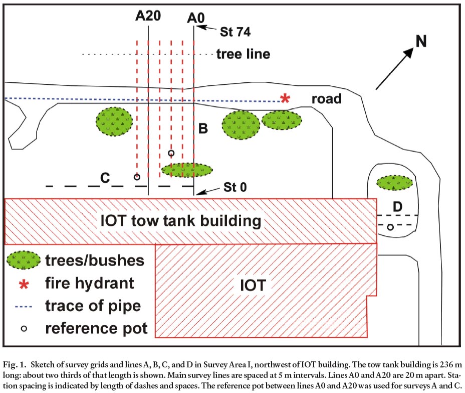
Survey Area II: SE of the Health Science Centre
13 The second field area is southeast of the Health Science Centre (HSC), bounded by Prince Philip Drive to the east, a pond to the west, and Clinch Crescent to the north (Fig. 2). In 1948, prior to major construction, the area consisted of marsh land. As roads were constructed, flooding recurred over Prince Philip Drive, and in 1992 BFL Consultants Limited was contracted by the city to construct a storm sewer system, which was completed in 1994. A 1.8 m diameter storm sewer, made of 2 mm-thick corrugated metal, runs through the field area at a shallow angle (about 15°) to Prince Philip Drive. In the central region, the pipe was laid near what was ground level at that time. The area is now a mainly grassy field, where the position of the buried pipe is indicated by a long mound, separated from Prince Philip Drive by a line of trees and a ditch about a metre deep.
Fig. 2. Sketch of Grid E, Survey Area II, southeast of the HSC, including line numbers (in meters from Clinch Cresent). SP profiles were measured with 4 m station spacings on unbroken lines. Station spacing is indicated by length of dashes on broken lines. Jogged line through middle of grid is the trace of a large-diameter storm sewer. Base line is 4 m (one dash length) southeast and parallel to the northeast trending part of the storm sewer. Reference pot position is indicated by the black open circle between lines 0 and 20.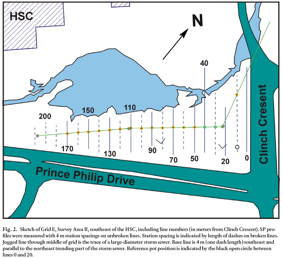
SURVEY SETUP AND PROCEDURES
Equipment
14 The equipment needed to carry out an SP survey consists of a high impedance voltmeter, wires, and non-polarizing porous pot electrodes. IP (induced polarization) receivers include SP capabilities, because SP voltages must be corrected for in IP surveys. For our surveys we usually used a Scintrex Model IPR8 IP receiver. For later surveys we used a Fluke 179 multimeter, which was much simpler to operate. The IP receiver had an internal offset bias. After compensating for this bias, the two instruments gave the same results, within the reading uncertainty of the IP receiver.
15 The electrodes are designed to minimize errors due to contact potentials between the electrodes and the ground. They consist of a ceramic cup (pot) filled with a saturated solution of CuSO4 (copper sulphate). The pot has a tight-fitting insulated lid and a porous base through which the solution seeps. To ensure good contact with the ground, grass and roots are cleared from immediately underneath the pot. On the top of the lid, wires are attached to an electrical connector which is in turn connected to a large, perforated copper cylinder which is immersed in the solution.
Setup for survey locations A-D, Survey Area I
16 Survey grid A, set up in the summer of 2005, consisted of two lines separated by 20 m bearing 134°, perpendicular to the IOT tow tank building. Line A0, station 0 was located 1.4 m from the wall of the building, 80.1 m from the northeast corner, and station numbers increased up to station 74, with a spacing 2 m (see Fig. 1). Line A20 was parallel to line A0 to the southwest. The location of the reference pot (see Procedure for Surveying) was midway between line A0 and A20 approximately 20 m away from the IOT building.
17 Survey grid B was set up by students of an undergraduate geophysics course in the fall of 2005 in the same area behind the IOT building. This grid was made up of 6 lines that were 5 m apart, so that lines B0 and B20 overlapped with lines A0 and A20. The lines ran from station 8 to station 68 with 2 m station spacing. (The station numbering corresponded to that of lines A0 and A20.) The reference pot was located on line B25, station 8.
18 Two additional, smaller surveys were undertaken in this region. Line C ran parallel to the IOT building and about 5 m away; it extended 65 m with station spacing 5 m. Grid D consisted of two lines perpendicular to the IOT building, but on the northeast side and close to the corner (Fig. 1). Line D3 started 7.2 m from the corner and Line D0 was about 4 m further. The lines were 16 and 18 m long. Station 0 was 15 cm from the concrete foundation of the building, and the reference pot was stationed 6 m from the wall and 1 m SE of line D0.
Setup for Grid E, Survey Area II
19 Grid E, set up in the Fall of 2005, consisted of 21 lines 10 m apart (Fig. 2). The bearing of the base line was 47°, parallel to the storm sewer and 4 m to the southeast. Stations were every 4 m, labelled negative to the northwest and positive to the southeast. Line E0 was 4 m from the edge of the road, Clinch Crescent. Magnetic and terrain conductivity surveys were completed on every line, whereas the SP survey was done on approximately every second line. The reference pot was located on line E10, station 30.
Procedure for surveying
20 Before surveying, the porous pots were soaked in CuSO4 for at least 40 minutes to make sure that the solution had seeped through the porous base of the pots. During the survey one electrode was kept at the reference location while the other ‘roving’ electrode was moved along a series of stations and lines and the potential difference between them was measured. Starting one minute after placement of the pot, two to four measurements were taken at each station over a period of 12 minutes. In some cases the instrument was turned off and on again. Mostly the reading did not change, but changes of 3 to 4 mV were not uncommon.
21 When surveying Grid A, a second reference location on line A0 station 30 was chosen in some cases, in order to monitor changes in the potential gradient across the grid.
Other geophysical techniques
22 Over grid B in Survey Area I and grid E in Survey Area II, surveys were undertaken with other geophysical instruments, including a terrain conductivity meter (Geonics EM31), a proton magnetometer (Scintrex ENVI MAG), and a ground penetrating radar (RAMAC/GPR).
23 The EM31 works by the principle of induction, and consists of a transmitter and receiver coil separated by 3.66 m (12 feet). The instrument can be carried at different heights above the ground, and can be orientated in two different configurations, with the plane of the coils perpendicular (HMD = horizontal magnetic dipole) or parallel (VMD = vertical magnetic dipole) to the ground. For horizontally stratified ground of low to moderate conductivity (normal rocks and soils) the EM31 measures a depth averaged electrical conductivity of the subsurface in milliseimens per metre. The median depth, above which (for ground of uniform conductivity) half the signal is received, is about 3.2 m for the VMD configuration and 1.4 m for the HMD configuration. The height at which the instrument is carried is included in these depths (Kearey et al. 2002). When traversing good conductors, such as metallic pipes, quantitative measurements are not obtained. Instead, a profile across a buried pipe will show a conductivity ‘high’ centered on the pipe or, for shallow burial depths, the ‘classic’ pipe signature of two ‘highs’ on either side of a central low (Reynolds 1997).
24 The magnetometer measures the total static magnetic field in nanoteslas (nT), and the vertical magnetic gradient in nT/m. The GPR consists of a transmitter that radiates short pulses of high frequency (10–1,000 MHz) radio waves into the ground and a receiver that records the reflected signal. The propagation of the signal is dependent on the dielectric constant and conductivity of the ground.
RESULTS
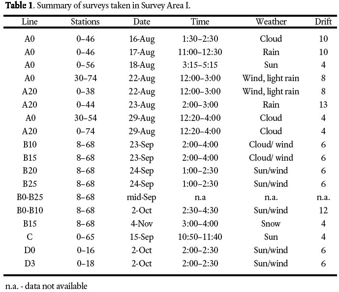
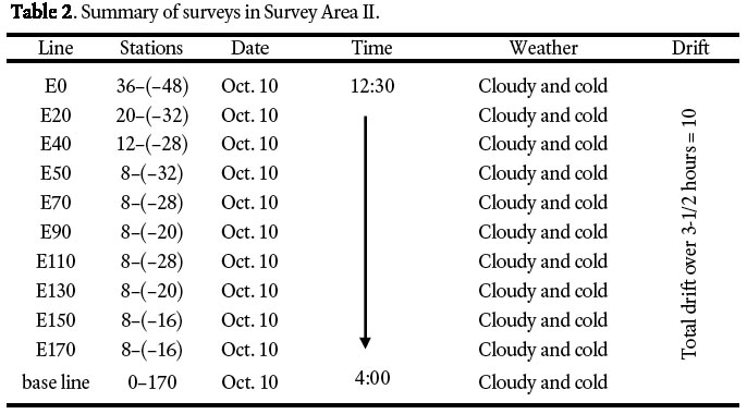
25 The data collected from the two survey areas are presented in a series of profiles (Figs. 3–6, 8–15, 19, 20). Tables 1 and 2 contain key information on the survey grids and lines including: lines, stations, date, time frame over which measurements were taken, weather, and measurement drift. The drift is the measurement difference recorded at the reference location over the given time frame.
Table 1. Summary or survey's taken in Survey Area I.
Display large image of Table 1
Table 1. Summary or survey's taken in Survey Area I.
Display large image of Table 2
Line A0
26 Figure 3 shows profiles of line A0 (Fig. 1) measured on four different days in 2005. For ease of viewing, the profiles have been graphically offset from one another by 50 mV. The closed symbols indicate a traverse toward higher station number, and the open symbols a subsequent traverse in the opposite direction. The data show an overall increase in potential away from the IOT building, to about station 38, and a series of excursions which are seen as negative anomalies at stations 8–10, 18, 26–28, 42–44, 56–58, and 70.
27 The difference between station 0 and station 30 is a measure of the potential gradient away from the building. On the three consecutive days (August 16, 17, and 18, 2005) this difference was 145, 170, and 140 mV corresponding to a gradient of 4.8, 5.7, and 4.7 mV/m. The magnitude of the anomaly associated with the water pipe (Stations 42–44) was measured by subtracting the high value at station 38 from the low value at station 42 or 44. On August 17, 18, and 22, values of 118, 38, and 51 were obtained. We note that the largest anomaly occurred on the same day, August 18, as the strongest gradient away from the building.
28 Of the six "anomalies" mentioned above, the negative peak at stations 8–10 can be correlated with a line of trees and that between stations 42–44 to the buried water pipe. The other anomalies are probably due to natural (non-anthropogenic) charged interfaces, such as the surfaces of boulders or changes in soil composition (see below).
Fig. 3. SP profiles of line A0 (Fig. 1) measured on 4 different days in August, 2005. Closed symbols, traversing to higher station numbers; open symbols, returning to lower station numbers. Actual potentials are given for profile 8/16/05. Other profiles are progressively offset by +50 mV. The thick dash indicates the approximate position of the buried pipe.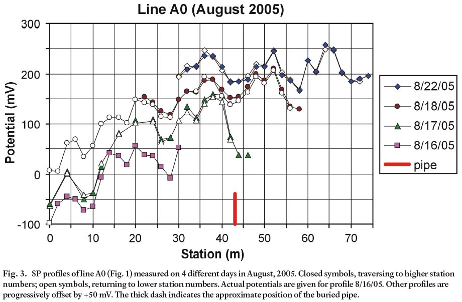
Display large image of Figure 3
Drift and repeatability
29 As can be seen by comparing the forward and reverse traverses in Fig. 3, the basic shapes of SP profiles are consistent over the period of the survey. However, the variations were significantly greater than the reading uncertainty of the instrument (1–2 mV). Figure 3 and Table 1 show that drifts of 5–10 mV over an hour or two were common. The shape of the profiles is also consistent from day to day, though the variations are larger.
GPR profile
30 Figure 4 shows GPR data along line A0 between stations 12 and 70. A marked diffraction hyperbola corresponds to the water pipe at station 44. Measurement of the asymptotes to this hyperbola gives a depth of burial for the pipe of about 21⁄2 m, which is to be expected as water pipes are generally located just below frost level, which is around 2 m. Numerous other, less distinct, diffraction hyperbole are probably due to boulders in the till. At very shallow levels (1–2 m), features in the GPR signal near stations 18 and 28 are coincident with SP anomalies. A diffraction hyperbola under station 28 suggests that this feature is due to a boulder. Those under station 18 may be due to variations in the layering or composition of the subsurface. Other features of the GPR section are a shallow-dipping reflector at about 4 m depth between stations 32 to 52, a steeper reflector at 10–12 m depth between stations 27 and 37, and changes in the ‘texture’ of the shallow subsurface below station 25 and above station 58. The shallow reflector presumably indicates layering in the glacial till. The deeper reflector may indicate bedrock. The textural differences below station 25 may be related to ground disturbance in the construction of the building, and that above station 58 to the presence of trees.
Fig. 4. GPR profile of line A0 (Fig. 1) taken Oct 4, 2005. A refraction hyperbole due to the water pipe shows clearly at station 44.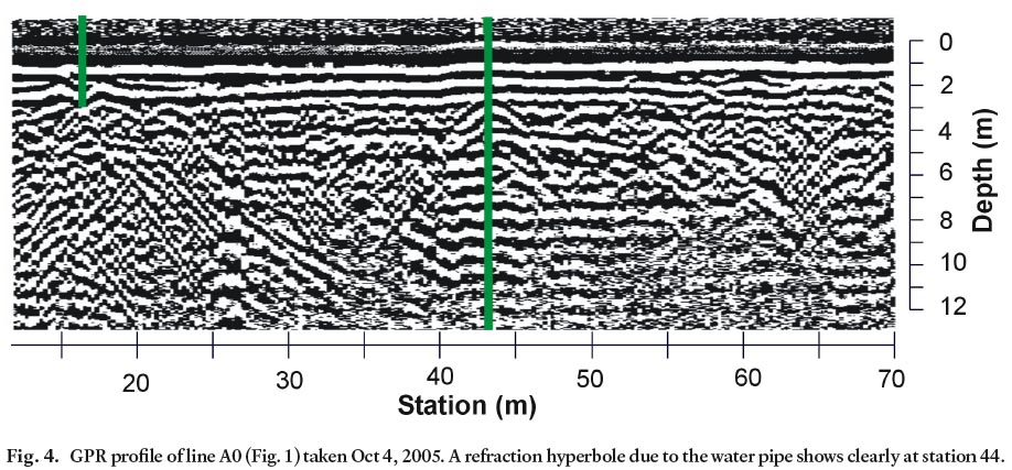
Ground conductivity readings
31 Profiles of ground conductivity along line A0 measured by the EM31 are shown in Fig. 5. For the VMD data, the median depth is approximately the same as the burial depth of the water pipe, so it is not surprising that this profile is dominated by a classic ‘pipe’ signature of a low surrounded by two highs. (This signature confirms that the water pipe is made of conductive iron.) Our instrument was incapable of recording negative numbers, so the central low registered as zero. The median penetration depth in the HMD configuration was about 0.6 m, so the water pipe did not register. The VMD data indicates that the ground northwest of the road is more conductive than that closer to the building, a feature that is also shown by the HMD data. Consistent with this result, the ground to the north is damper and more highly vegetated.
Fig. 5. Ground conductivity profiles taken using the Geonics EM31 held at hip level. The median penetration depth below the surface is about 2.4 m in the VMD configuration, and 0.6 m in the HMD configuration.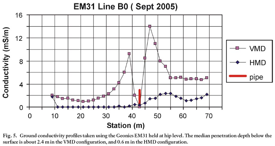
Display large image of Figure 5
32 Superimposed on the signals due to the water pipe and variations in ground conductivity is a secondary peak in conductivity between Stations 50 and 55. This peak may indicate the presence of another, less conductive, perhaps highly corroded pipe. Though the GPR profile is inconclusive, the existence of a second pipe is supported by the SP profiles (Fig. 3) and the magnetometer readings (Fig. 9).
33 In 2004, the conductivity profiles gave similar shapes but higher values (in particular, HMD values south of the road were between 1 and 2 mS/m), perhaps because there had been more rain in September that year.
Line A20
34 The three upper profiles in Fig. 6 were measured along Line A20 in August, 2005. The two profiles measured on August 23rd and 29th show, like the profiles of Line A0 in Fig. 3, that the basic shape of the SP signal is constant over a period of days. However, the profile measured on August 22nd shows entirely different anomalies. Although the positive slope in potential away from the building is very similar to that of the profile taken a week later, the smaller anomalies are different; in fact, negative anomalies at stations 2, 14, 22, 28, and 36 and positive anomalies at stations 20 and 26 appear to have either disappeared or, more commonly, been replaced by an anomaly of the opposite sign. The two short transects from Line A0 taken on the same two days show similar behaviour; the signal from the water pipe, which on August 22nd was a significant negative anomaly, became a small positive anomaly on August 29th. On Line A20 the pipe also generated a small positive anomaly on August 23rd and 29th.
Fig. 6. SP profiles of line A20 (Fig. 1) taken on 3 different days in August, 2005. Potential values apply to profile 8/22/05. Profiles 8/23/05 and 8/29/05 are offset by 50 and 100 mV respectively. Also shown are two profiles over the water pipe on line A0. Profiles 8/29/05(A0) and 8/22/05(A0) are offset by –100 mV and –170 mV, respectively.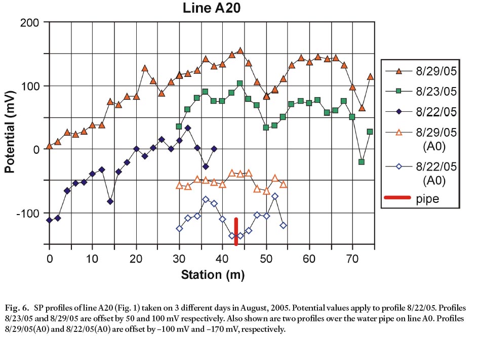
Display large image of Figure 6
35 What happened between the 22nd and the 23rd of August? Figure 7, a plot of the daily rainfall in St John’s during August, suggests that soaking of the ground with rain is likely to be the cause of the change in the SP signal. After 3 weeks of relatively warm, dry weather, August 23rd heralded four days of significant rainfall. The rain evidently had little effect on the signal from the IOT building, which may be related to chemical potentials between the earth and its deep foundations, while profoundly affecting the smaller near-surface charge concentrations. It is noteworthy that while the electrochemical conditions around these small ground features changed when they were soaked with rainwater, the features themselves were not ‘washed away’.
Fig. 7. Total daily rainfall and mean temperature recorded at St John’s airport during August, 2005. Data are from Environment Canada (2005).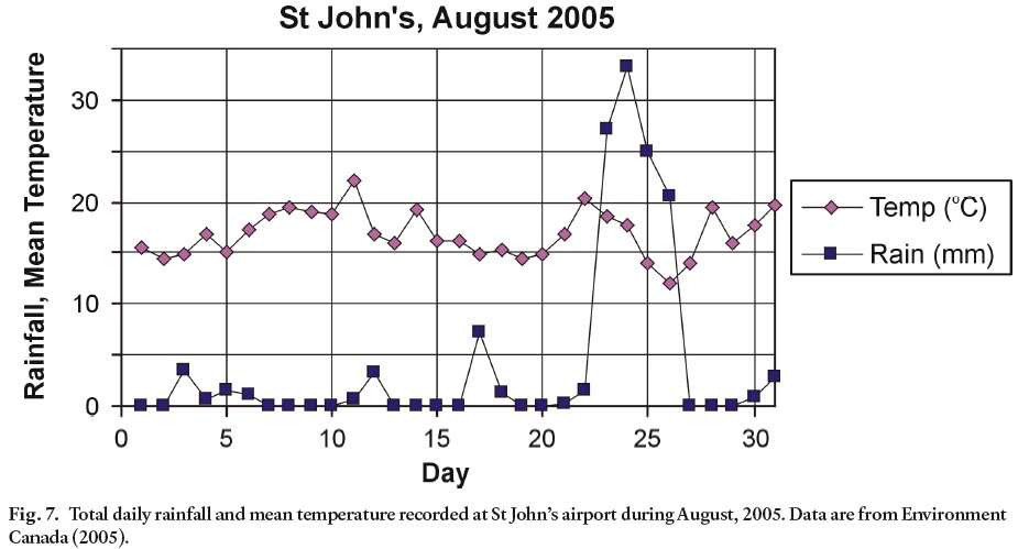
Grid B
36 Lines surveyed within Grid B by an undergraduate class over a period of 3 weeks in September are shown in Fig. 8. Because the lines were not surveyed on the same day, and the stations along B0 and B20 do not coincide with those of A0 and A20, detailed comparisons are not warranted, but some general comments can be made.
Fig. 8. SP profiles of Grid B (Fig. 1) taken on different days in September, 2005. Missed readings on Line B25 correspond to a large puddle on the road.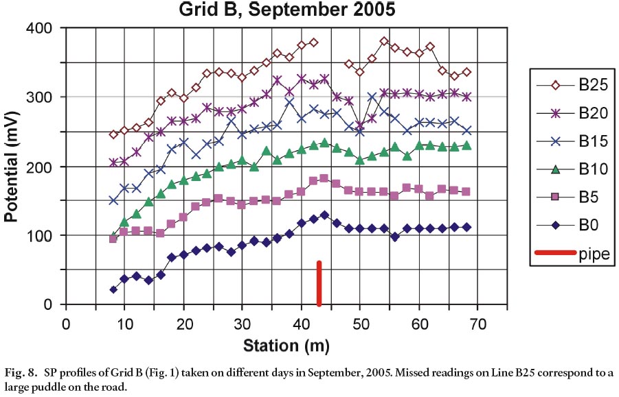
Display large image of Figure 8
37 The lines are sub-parallel, the potential rising away from the building to about station 40, where the influence of the water pipe is felt. Lines B0 and B5 show elevated readings at stations 8 to 12 corresponding to the clump of trees parallel to the IOT building (Fig. 1). A big dip in the potential occurs on the far side of the road on Lines B15 to B25, similar to that observed on Line A20 (Fig. 6). This dip may be related to the ground there being particularly wet, as indicated by the occasional presence of a large puddle on the road, or it could be related to the presence of a second pipe. Alternatively, both positive and negative peaks may be due to the pipe (see below, Modelling of Charge Distribution on Storm Sewer and Fig. 20).
38 The small anomalies (apart from those due to the pipe and the trees) do not line up; for example, small positive anomalies at Stations 20, 28, and 38 of Line B15 are not seen on the other lines. Evidently the anomalies are isolated and do not run parallel to the building. The comparative ‘bumpiness’ of Line B15 was observed the previous year (though, again, the stations were not in exactly the same locations). Line B0 appears to be somewhat smoother than Line A0 in Fig. 3: in particular on the northeast side of the road Line B0 is very flat. We will return to these observations later.
Magnetometer readings
39 Figure 9 shows profiles of the total magnetic field on Grid B. The main features are a pronounced low extending at least 30–40 m along each line from the IOT building, and a smaller amplitude high at station 46–50 followed by a low about 8 m farther along each line. In St John’s at the time of the survey, the geomagnetic field had a declination of 20.5°, inclination of 68° and intensity of 51,700 nT (e.g., National Geophysical Data Center 2006). For a localized object magnetized by this geomagnetic field, the anomaly expected is a pronounced high to the (magnetic) south and a smaller low to the north. Profiles of the magnetic field over the storm sewer in Grid E (Fig. 15) display this expected shape. The wide, high amplitude low seen at low station numbers in Grid B is also well explained by geo-magnetization of the IOT building. The smaller amplitude peak and trough seen in Grid B has the shape produced by a buried, magnetized pipe; however, it is offset 6–8 m to the northwest from the known position of the fire hydrant pipe. It may be that the signal is due to another pipe under station 52 (see EM31 data, Fig. 5) and that the small diameter fire hydrant pipe does not generate a significant magnetic field.
Fig. 9. Profiles of total magnetic field on Grid B, taken on various days in September, 2005. Values on vertical axis apply to profile B0. Each overlying profile is further offset by 500 nT.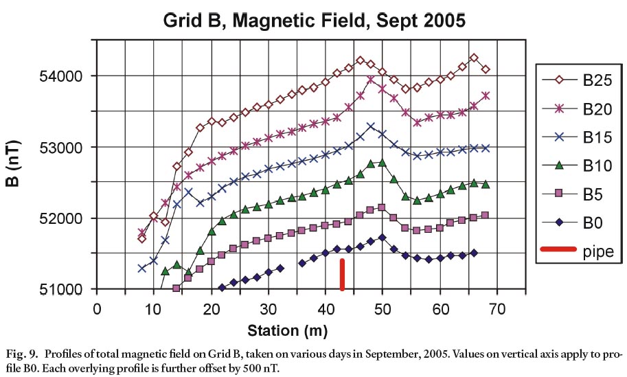
Line C and Grid D
40 Line C and Grid D (see Fig. 1) were surveyed to check that the IOT building was responsible for the large-scale negative anomaly seen at low station numbers in Lines A and Grid B. Figure 10 shows a profile of Line C, parallel to the IOT building. As expected, the readings show much less variation, only about 20 mV, than those perpendicular to the building (Lines A and B) and no overall trend. Higher values on Lines 5 and 10 may be related to the nearby clump of trees.
Fig. 10. SP profile along Line C, parallel to the IOT building at a distance of 5.4 m, along station number 4 of Grids A and B. Station 0 is on Line A0, and Station 20 is on Line A20. Closed symbols are for a traverse in ascending station numbers. Open symbols indicate a return traverse in the opposite direction.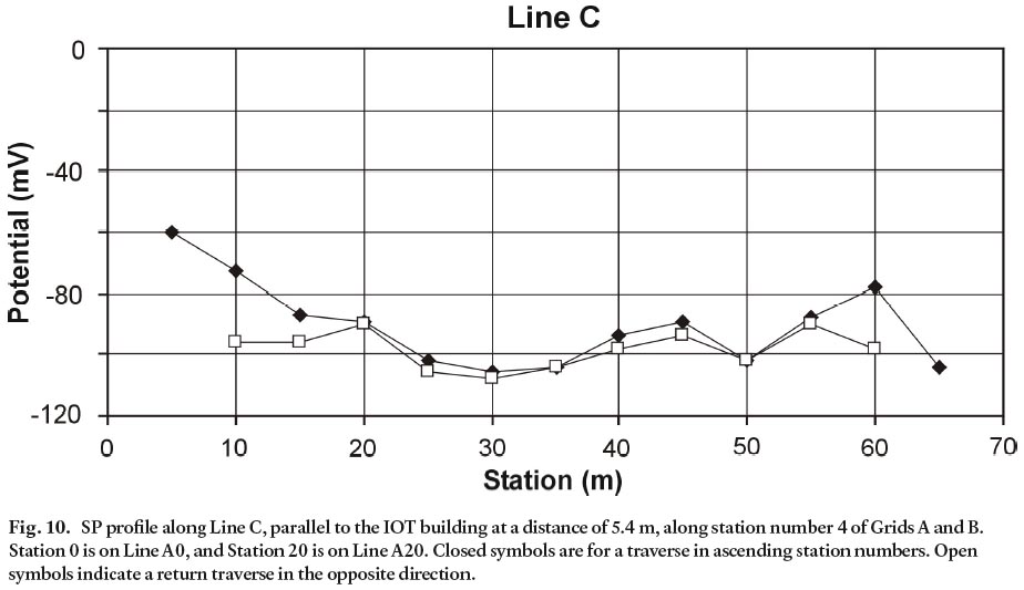
Display large image of Figure 10
41 Grid D consists of two lines perpendicular to the building, on the northeast wall and closer to the corner than Lines A0 and A20 and Grid B (Fig. 1). The profiles (Fig. 11) support the building having a negative charge. The potential rises quasi-linearly away from the building, as it does in Lines A and Grid B. The gradient, measured between stations 0 and 10, is 12 mV/m, about twice that observed on the northwest wall. This difference is consistent with the more rapid change in potential expected near the corners relative to the sides of charged objects. The total change in potential of 120 mV is similar to that observed away from the northwest wall (Fig. 6).
Fig. 11. SP profiles of lines D0 and D3 (Fig. 1), measured on October 2, 2005.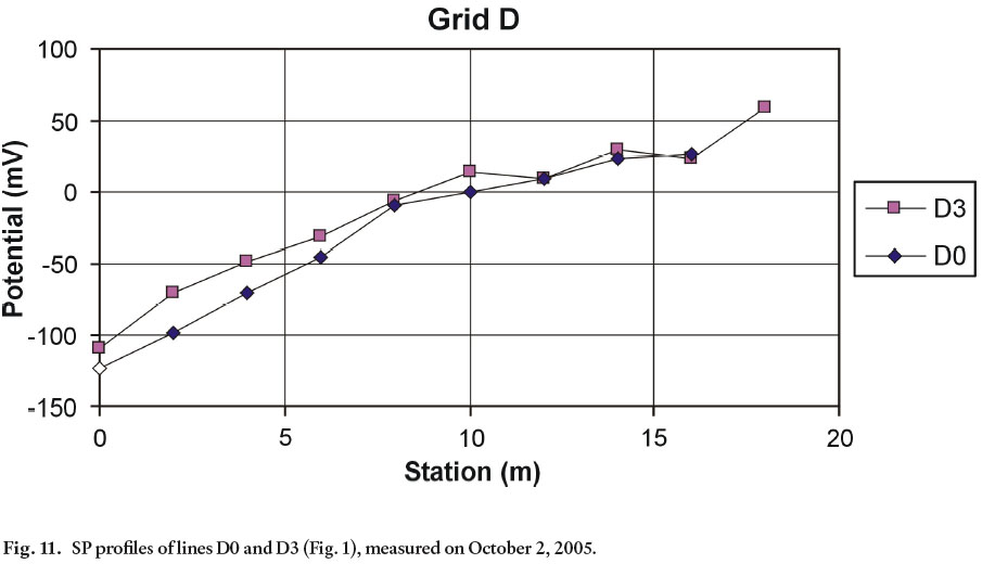
Grid E
42 In Grid E, Survey Area II, SP profiles with 4 m station spacing were measured on 10 of the lines (unbroken lines on Fig. 2). The dominant ground features in this area are a 1.8 m-diameter storm sewer pipe and associated manholes with square metal covers located at about lines 23, 108, and 195. Two other round metal covers are located at about line 50, station 2 and line 155, station 2.
43 Figure 12 shows that there is a significant SP anomaly directly above the sewer pipe. This anomaly is on Station 4 on all lines except E20 where the anomaly occurs on Station +4 because the pipe bends to the north (see Fig. 2). The anomaly is negative (50–80 mV) on most of the lines, but is even larger and positive on lines 110 and 170. The anomaly on line 110 (165 mV) is probably associated with the nearby manhole, which is a substantial structure. The other positive anomaly could be related to a difference in the soil compositions around the pipe. The plans for placement of the pipe (BFL Consultants Ltd, 1993) show the area around Line 170 as about 1.5 m lower in elevation than the surroundings, and slated for infilling with topsoil. From Lines 160 to 45, the plans show the sewer pipe lying on the existing surface with topsoil and sod to be added around and on top of it to a depth of 50 cm. Below Line 45, up to 50 cm of excavation was required.
Fig. 12. SP profiles on Grid E, October 10, 2005. Values of potential on vertical axis apply to line E20. Overlying lines are successively offset by 50 mV.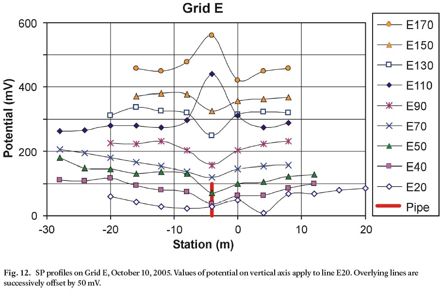
Display large image of Figure 12
44 Figure 13 displays profiles of the potential parallel to the sewer pipe on stations 0, 4, and 16. These profiles are not offset from one another, so the lower potentials on Line 4 are real and due to the charge on the storm sewer (Fig. 12). The positive anomaly associated with the manhole near Line 110 is quite localized; it is 240 mV on Line 4, 50 mV on Line 0, and not present on Line 16, 12 m from the manhole. The positive anomaly on Line 170 is asymmetric so that it does not appear as an anomaly along Station 0 (Fig. 13), but judging from Fig. 12 it has a similar width to that on Line 110. The potentials on Line 0 are not related to the storm sewer (see Fig. 2). They are probably affected by electrical wiring and a water main which run along the southwest edge of Clinch Crescent.
Fig. 13. SP profiles approximately parallel to the sewer pipe in Grid E, along the stations indicated. Station 4, from Line 20 to 170, is on top of the pipe. Lines are not offset.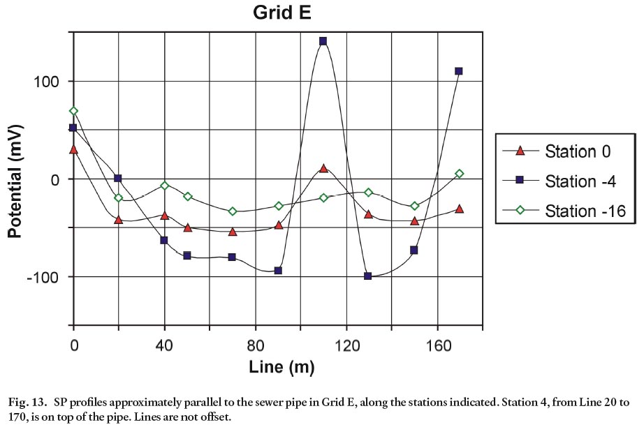
Display large image of Figure 13
Ground conductivity and magnetics
45 Two representative profiles of apparent ground conductivity are plotted in Fig. 14. As for EM31 profiles in Grid B (Fig. 5), the data measured in the VMD configuration (which has a median sampling depth of 2.4 m) show the classic ‘pipe’ signature of two conductivity ‘highs’ surrounding a ‘low’, though the signature appears strongly asymmetrical, perhaps an artefact of the coarse sampling interval. The HMD shows a conductivity high which is offset, as it is on Line B0 (Fig. 5), perhaps because the ground is more conductive under the more negative stations. Alternatively, this offset and the asymmetry of the VMD signal may be related to topography.
Fig. 14. Ground conductivity profiles taken using the Geonics EM31 held at hip level on Line E130.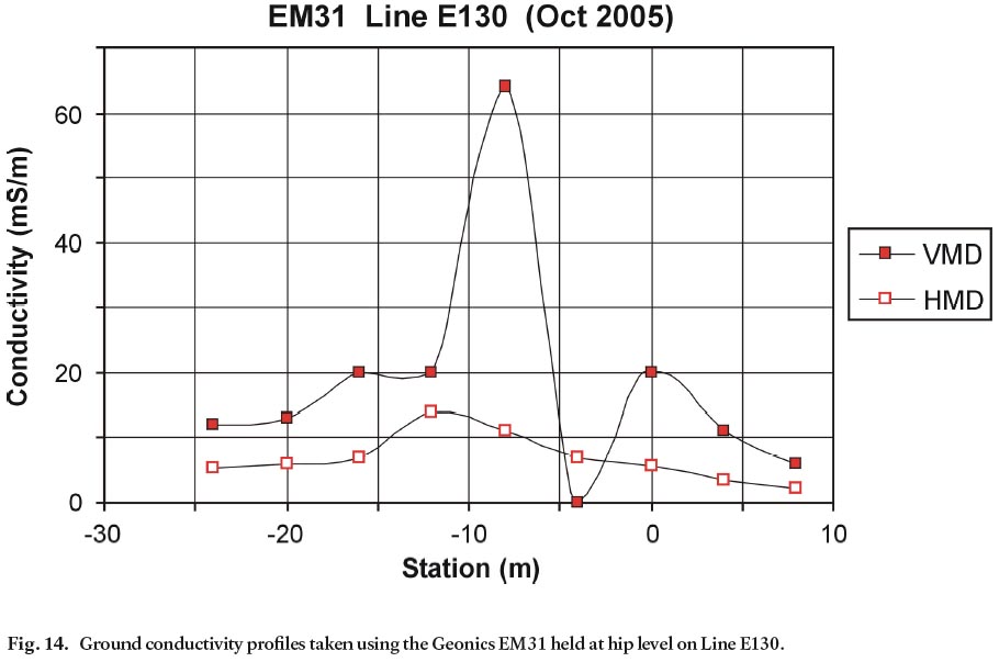
Display large image of Figure 14
46 Figure 15 displays the total magnetic field on selected lines of Grid E, measured by the ENVIMAG magnetometer. The pattern of a large high to the south of the pipe and a less pronounced low to the north is exactly what is expected over a pipe magnetized by the Earth’s field in northern mid-latitudes. The centre of the storm sewer is located approximately midway between the high and low. The more complex pattern on Line E20 is due to the influence of the nearby manhole.
Fig. 15. Profiles of total magnetic field on selected lines of Grid E, October, 2005. For ease of viewing, successive profiles are offset by 800 nT.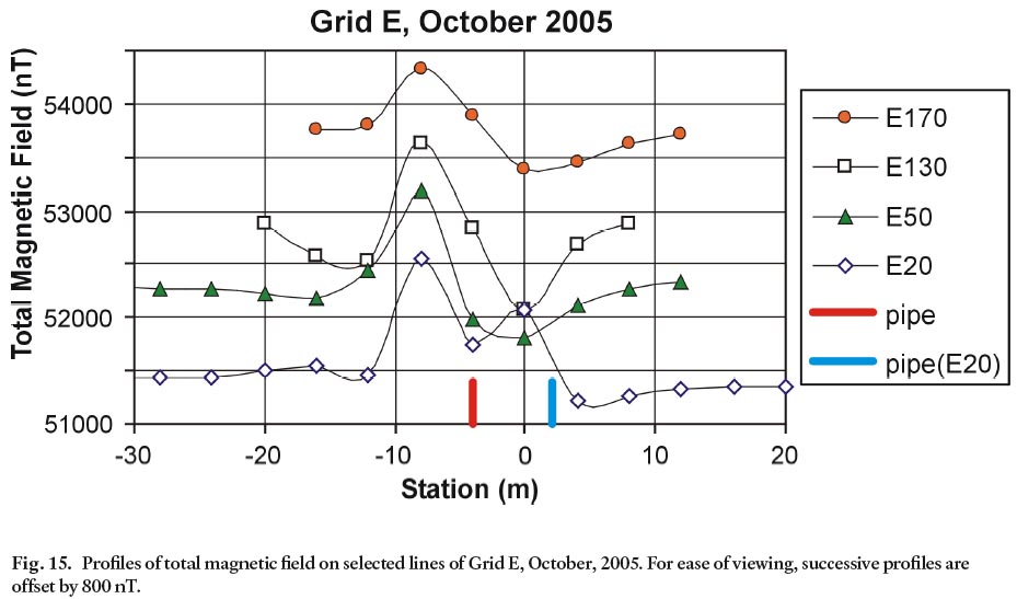
Modelling of charge distribution on storm sewer
47 The regular distribution of potential over the storm sewer encouraged the authors to undertake simple mathematical modelling of its electrical charge. The small number of data points defining the profiles precluded complex modelling. The pipe is long compared to its diameter, and over most of its length the potential is symmetrical, and of the same sign and similar magnitude. The simplest charge distribution that fits these observations is a uniform surface charge σ0 C/m2 on the outside of the pipe. The resulting potential can be found by a simple application of Gauss’s Law (e.g., Griffiths 1999). As a function of distance x along a traverse perpendicular to a pipe buried a distance z below location x = 0, this potential is

48 The next simplest charge distribution is a dipole surface charge, which varies with the cosine of the azimuthal angle, φ, measured from the vertical around the pipe.

49 The resulting potential on a traverse over the pipe is:

50 Figure 16 shows SP profile E130 and examples of calculated profiles over a uniformly charged pipe at three different burial depths, z = 1, 2 and 4 m. From the building plans (BFL Consultants Ltd, 1993) the centre of the storm sewer was originally at a depth of about 1.4 m. For any burial depth, a fit can be found for the three points closest to the pipe, but none of the profiles fits the data farther away. Our observations require a profile which flattens out only a few metres from the pipe, whereas the potential due to a uniformly charged pipe will change monotonically over a horizontal distance comparable to the length of the pipe, which in the case of the storm sewer is at least tens of metres.
Fig. 16. Calculated potential on a traverse over a long pipe with uniform charge per unit length for 3 different burial depths, z. Corresponding surface charges are (assuming radius R=0.9 m): –0.45 (z = 1 m), 0.79, and 1.84 pC/m2. Reference distances r0 are 9, 7, and 6.85 m, respectively. Also shown is measured profile E130 over the storm sewer.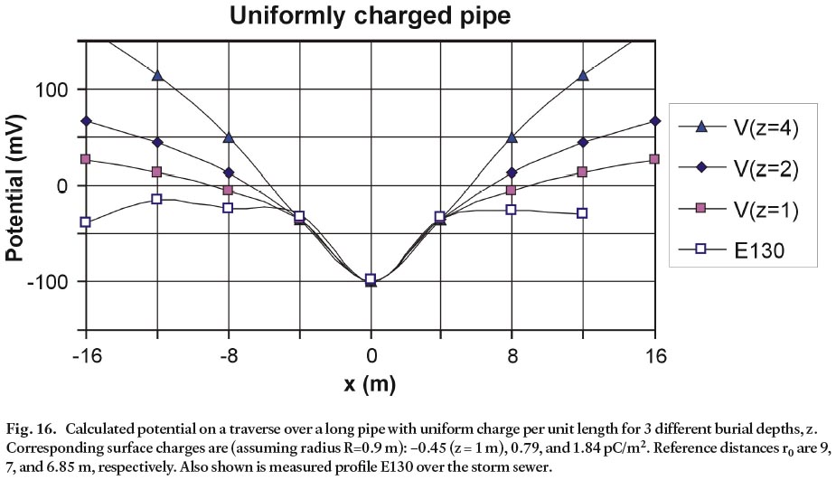
Display large image of Figure 16
51 Calculated profiles over a pipe with a cosine distribution of charge for the same burial depths are shown in Fig. 17. The dipole moment here is pointing vertically downward: in other words, the maximum negative charge density is on the top of the pipe. These profiles have the desired shape to fit SP profile E130, and the best fit width corresponds to a realistic burial depth of between 1 and 2m. Thus, a cosine variation of charge around the pipe (or at least one in which positive and negative charges are separated over the pipe but in balance overall) appears to be a good first order approximation for profile E130.
Fig. 17. Calculated potential on a traverse over a long pipe with cosine surface charge (Eqn (2)) for 3 different burial depths, z. Corresponding values for σ0 are (assuming radius R=0.9 m): –0.875 (z=1 m), –1.75, and –3.5 pC/m 2. Potential offset V0 is 20 mV. Also shown is measured profile E130 over the storm sewer.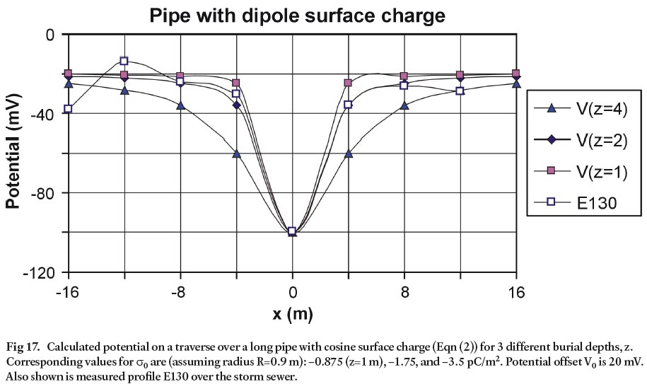
Display large image of Figure 17
52 Some of the other profiles (e.g., E170 and E50, Fig. 12) are not as symmetrical and the fit is improved if the dipole moment is tilted at some angle φ0. The potential along a traverse is (e.g., Satyanarayana Murty and Haricharan 1985).

53 Figure 18 shows representative profiles calculated from Equation (4). Tilt has the effect of moving the peak anomaly to one side of the pipe, rather than directly above it, and introducing a smaller anomaly of opposite sign on the other side of the pipe. The profiles are qualitatively similar to those over the tilted magnetic dipole field of the pipe (Fig. 15), although the equations are not exactly the same.
Fig. 18. Calculated profiles over pipes with cosine surface charge distributions (Eqn (2)), where the dipole is tilted at angle phi0 (φ0) to the vertical. Calculations use Eqn (4) assuming R=0.9 m, σ0=1 pC/m2, and z=1.5 m.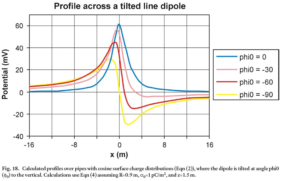
Display large image of Figure 18
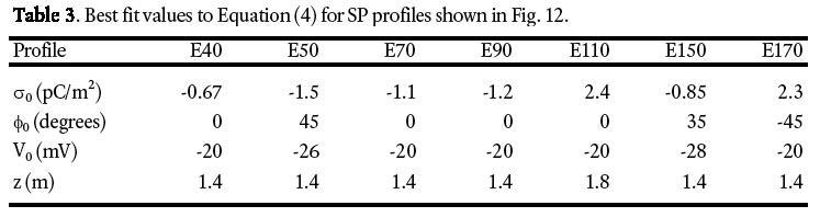
54 Table 3 shows values of σ0 and φ0 which give reasonable fits for the profiles shown in Fig. 12. Only profile E70 is better fitted by a combination of dipole and uniform charges; however, it is also possible that the profile is affected by charges other than those associated with the storm sewer.
Table 3. Best fit values to Equation (4) for SP profiles shown in Fig. 12
IOT revisited in 2006
55 In May and June 2006, repeat surveys were carried out of some of the lines in Grids A and B, behind the IOT building. For Line A0, shown in Fig. 19, the readings were taken at exactly the same stations nearly a year apart. Each profile is an average of readings taken on two different days. Although there were day-to-day differences in the readings (e.g., see Fig. 3), these differences are small compared with those observed over the 101⁄2 month time interval.
Fig. 19. Comparison of profiles along Line A0 on August 18th and 22nd, 2005, during dry, warm weather, and June 2nd and 5th, 2006, when the weather was cool and damp.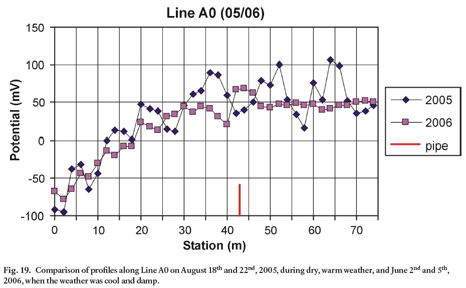
Display large image of Figure 19
56 We note first that the overall shape of the profiles, including the gradual increase in potential away from the building for the first 30 m followed by a flattening of the potential, is the same. The profiles are not offset or scaled: they really do fall on top of one another. A distinct anomaly is associated with the water pipe, although the anomaly is negative in August 2005 and smaller and positive in June 2006. The pattern of the 2006 profile up to station 25 is a smoothed and muted version of the 2005 profile: steep changes between stations 2–4, 8–12, and 18–20 have the same direction but smaller magnitude in the later year. The correlation between the surveys from station 26 to station 74 is poorer. North of the road, beyond station 50, the 2006 profile is very smooth, as was observed also on Line B0 in September 2005 (see Fig. 8).
57 A comparison between the first three lines of Grid B surveyed in September 2005 and June 2006 is plotted in Fig. 20. On a scale of about 10 m, the features of these profiles correlate well with each other. All of these profiles show the water pipe giving a positive anomaly, though the shape and magnitude of the anomaly varies. The localized nature of the anomaly suggests that there is a dipole rather than a uniform charge on the water pipe, as there is on the sewer pipe in Grid E (see Figs. 17 and 18), and the shapes of the profiles over the pipes suggest that the dipole charge is in some cases tilted (e.g., compare B0 (06) in Fig. 20 with profiles in Fig. 18). A dipole model was fitted to one of the smoother profiles, B5 (06), and gave a reasonable fit to the data for a pipe at a depth of 2.5 m. Given a pipe radius of about 15 cm, standard for the fire hydrant water pipes on the Memorial University campus (C. Chaytor, Facilities Management, Memorial University, personal communication), the maximum charge density ± σ0 was 40 pC/m2, about 40 times that of the storm sewer pipe in Grid E. This difference may indicate a higher corrosion rate. The high corrosion rate of iron in certain environments is one reason that some modern water pipes are made of plastic, or encased in polyethylene (Ductile Iron Pipe Research Association 2005). Metal pipes are not encased on the Memorial University campus, and corrosion of pipes laid in the 1970s has been observed in boggy ground around the Health Science Centre. The state of the pipe behind the IOT building is unknown; corrosion problems are only detected when the pipes leak.
Fig. 20. Profiles in Grid B taken on September 2005 (closed symbols) and June 5th, 2006. 2005 profiles are offset from B0(05) by 75 mV, 2006 profiles by 85 (B0-B5), and 75 mV (B5-B10). B0 (06) is subset of Line A0 (2006) in Fig. 19. B0 (05) may be offset 2 m relative to B0 (06).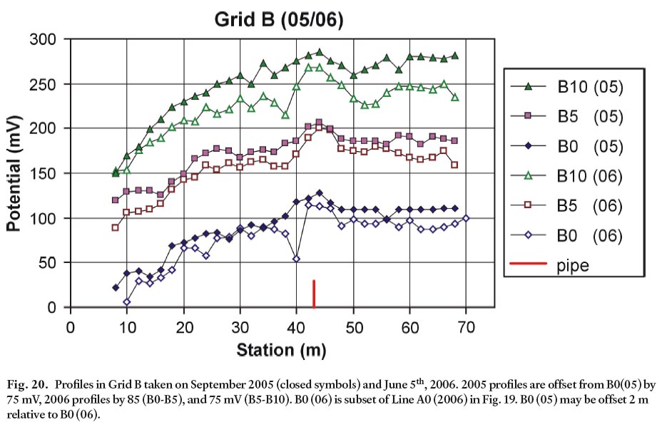
Display large image of Figure 20
58 It was suggested earlier that changes in sign and magnitude of anomalies due to the pipe and other small ground features were related to the weather. When the profiles between August 16th and 22nd , 2005, were taken, short-wavelength SP anomalies were relatively large (~50 mV), the water pipe generated a large negative anomaly of 50–100 mV (Fig. 3), and the weather had been warm and dry for the previous three weeks (Fig. 7). Data collected at other times (Figs. 8, 19, and 20) show short-wavelength anomalies in the range of only 10–20 mV and the water pipe associated with a positive anomaly of 20–50 mV. Undergraduate reports of geophysical surveys in September of previous years indicate that the anomaly is usually positive. Figure 21 shows that the weather prior to the June 2006 profiles was much cooler and wetter than the previous early August. As the weather in St John’s is usually cool and wet, it is suggested that the SP profiles in Fig. 20 are more typical of the area in the Fall than those in Fig. 3.
Fig. 21. Total daily rainfall and mean temperature recorded at St John’s airport during late May and early June, 2006. ‘Day’ is relative to the start of May, so June 2nd and 5th are days 33 and 36. Data from Environment Canada (2006).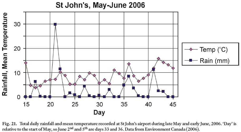
DISCUSSION AND CONCLUSIONS
59 In the present study, we compared the results of small-scale SP surveys in two open areas of the Memorial University campus with those of other geophysical techniques, including ground-penetrating radar (GPR), ground conductivity (EM31), and magnetics. We found that all the techniques responded well to the main, anthropogenic ground features. Each technique responded to a contrast in physical properties between the (usually metallic) anthropogenic features and their surroundings, such as magnetization, conductivity, dielectric constant, or charge build-up around the bodies.
60 The magnetic and ground conductivity data are smoother than the SP data, with no signals corresponding to the small, short-wavelength SP anomalies (cf. Figs. 5 and 9 with Fig. 6). The smoothness is reasonable given that the ENVIMAG and EM31 signals are averages over several metres in all directions in the subsurface, whereas the SP measurements may indicate very local charge distributions. The GPR profile (Fig. 4) indicates that heterogeneities are present in the shallow subsurface of similar wavelength to the SP anomalies.
61 The SP signals around the buried pipes are due, to a first approximation, to equal and opposite charges distributed along and on opposite sides of the pipe. We interpret the charge separation as being due to differences in the redox potential between the pipe and the surrounding soil and groundwater. The sub-vertical orientation of many of the dipole moments would then be the result of stratified ground, or perhaps of by-products of pipe corrosion seeping downward in the groundwater on the outside of the pipe under gravity, and changing the redox conditions between top and bottom. For the storm sewer, the dipole moment changed sign between regions where the ground had been excavated to lay the pipe and regions where the ground had been infilled (Line 170, Fig. 12), consistent with the interpretation that nature of the surrounding soil influences redox potential. We also observed that the sign and magnitude of the dipole moment of the water pipe changed when the weather changed from warm and dry to cool and wet. In warm dry weather, larger anomalies were observed, consistent with higher ion concentrations and less continuity in the groundwater. Charges may build up, for example, between regions of damp, clay-rich soils and drier sandier soil. After significant rain, this type of anomaly would be reduced or eliminated (see Fig. 19).
62 In common with previous workers, we found many small (10–50 mV), localized (5–10 m) anomalies that did not correlate to any obvious changes in the surface, or with features in magnetic and ground conductivity surveys. The anomalies were consistent over days to weeks (Fig. 3) and at least some were consistent over many months (Figs. 19, 20), indicating that, whatever their source, they were not random. We attribute these anomalies to subtle ground variations such as changes in soil type, the concentration of plant roots or buried boulders. Glacial till in Atlantic Canada is full of such heterogeneities: it is possible that the bumpiness of SP profiles could be used as a measure of the heterogeneity of the shallow subsurface.
63 In addition to small spatial variations due to ground conditions, and time variations due to groundwater conditions, small fluctuations of a few mV in the SP signal were observed over a time scale of minutes to hours. These fluctuations are probably due to telluric currents which, when passing through non-uniform ground, would cause charges to build up on boundaries between materials of contrasting resistivity.
64 For mineral exploration, where anomalies associated with ores are typically several hundred millivolts, small spatial variations are ignored as noise, but this consistent sensitivity to small ground features is one of the strengths of the SP method in archaeological mapping and one reason SP is promoted for environmental monitoring (Nyquist and Corry 2002). However, the fact that the strength and even the sign of the anomalies might change with the weather, through its effects on groundwater, and with space weather, through its effect on telluric currents, means that care must be taken in making and interpreting maps. If small signals are of interest when making a map, then it is advisable to complete the survey in consistent weather conditions, and to have more than one reference electrode, so that changes in large-scale gradients can be monitored.
ACKNOWLEDGEMENTS
The authors thank M. Hassan for assistance in collecting data in 2006. The manuscript benefited significantly from thoughtful reviews by K. Howells, P. Ryall, and F. Marillier.REFERENCES
BFL Consultants Ltd. 1992. Health Science flooding remedial works, Prince Philip Drive, Project 75-53, Drawing W-C-1.2.
Bigalke, J., and Grabner, E.W. 1997. The geobattery model: a contribution to large scale electrochemistry, Electrochi-mica Acta, 42, pp. 3443–3452.
Corry, C.E.1985. Spontaneous polarization associated with porphyry sulfide mineralization. Geophysics, 50, pp. 1020–1034.
Davenport, G.C., Hadley, L.M., andRandall, J.A. 1978. The use of seismic refraction and self potential surveys to evaluate existing embankments. URL <http://www.heritagegeophysics.com/papers/dave6.htm>, July 2006.
Ductile Iron Pipe Research Association. 2005. URL <http://www.dipra.org>, October 2006.
Environment Canada. 2006. URL <www.climate.weatheroffice.ec.gc.ca/climateData>, October 2006.
Frasheri, A. 2002. Relations between the hydrocarbon migration chimney and the electric self-potential field. Journal of the Balkan Geophysical Society, 5, pp. 47–56.
Griffiths, D.J. 1999. Introduction to electrodynamics. 3rd edition. Prentice-Hall, Inc., New Jersey, 146 p.
Howells, K., and Fox, D. 1998. Geophysical methods for detecting shallow sulphide mineralization in the Halifax Formation, Nova Scotia: a reconnaissance study. Atlantic Geology, 34, pp. 211–227.
Kearey, P., Brooks, M., and Hill, I. 2002. An introduction to geophysical exploration. 3rd edition. Blackwell Science Ltd., London, 262 p.
King, A.F. 1988. Geology of the Avalon Peninsula, Newfoundland, (parts of 1K, 1L, 1M, 1N and 2C). Government of Newfoundland and Labrador, Department of Mines and Energy, Mineral Development Division, Map 88-01, scale 1:250,000
King, A.F., Anderson, M.M., and Benus, A.P. 1988. Late Precambrian sedimentation and related orogenesis of the Avalon Peninsula, eastern Avalon Zone. Geological Association of Canada, Field trip guidebook: Trip A4, St John’s, Newfoundland, 84 p.
Lorne, B., Perrier, F., and Avouac, J.-P. 1999. Streaming potential measurements 1, Properties of the electrical double layer from crushed rock samples. Journal of Geophysical Research, 104, pp. 17857–17877.
National Geophysical Data Center. 2006. Geomagnetism. URL <http://www.ngdc.noaa.gov/seg/geomag>, October 2006.
Nyquist, J.E., and Corry, C.E. 2002. Self potential: the ugly duckling of environmental geophysics. The Leading Edge, May 2002, pp. 446–451.
Panthulu, V., Krishnaiah, C., and Shirke, J.M. 2001. Detection of seepage paths in earth dams using self potential and resistivity methods. Engineering Geology, 59, pp. 281–295.
Park, S., Wolf, L.W., Lee, M., and Saunders, J. 2004. Self-potential and geochemical measurements of microbially mediated bacterial sulfate reduction in saturated sediments. American Geophysical Union, Fall Meeting 2004, abstract #B53A-0983.
Raven, A. 1999. A geological, geophysical and prospective report on the Tommy Jack Property, Omineca Mining Division, British Columbia. British Columbia Prospectors Assistance Program, Ministry of Energy and Mines, Geological Survey Branch, Report PAP 99-22, 81 p.
Reynolds, J.M. 1997. An introduction to applied and environmental geophysics. John Wiley and Sons, England, 796 p.
Sato, M., and Mooney, H.M. 1960. The electrochemical mechanism of sulfide self potentials. Geophysics, 25, pp. 226–249.
Satyanarayana Murty, B.V., and Haricharan, P. 1985. Nomogram for the complete interpretation of spontaneous potential profiles over sheet-like and cylindrical two-dimensional sources. Geophysics, 50, pp. 1127–1135.
Trique, M., Richon, P., Perrier, F., Avouac, J.P., and Sabroux, J.C. 1999. Radon emanation and electric potential variations associated with transient deformation near reservoir lakes. Nature, 399, pp. 137–141.
Wynn, J.C., and Sherwood, S.I. 1984. The self-potential (SP) method: an inexpensive reconnaissance and archaeological mapping tool. Journal of Field Archaeology, 11, pp. 195–204.
Zhou, X., and Herold, K.E. 2003. Streaming potential effects in flows on biochips. American Society of Mechanical Engineers, Bioengineering Division, Extended abstract, Summer bioengineering conference, June 25–29, Key Biscayne, Florida, USA, pp. 605–606.
Editorial responsibility: Sandra M. Barr