Volume 6, No. 2 December 2003

Neural Network Forecasting of the Production Level of Chinese Construction Industry

by
Dilli R. Aryal*
and
WANG Yao-wu
Harbin Institute of Technology, Harbin, 150001, China

Increased efforts have been devoted over the past several decades to the development and improvement of time series forecasting models. In this paper, we determine whether the forecasting performance of variables under study can be improved using neural network models. Among the best 10 retained networks, an MLP 3- layer network: 1:1-31-1:1 is selected as the ANN model with the minimum RMSE. The performance of the model is evaluated by comparing it with the ARIMA model. The root mean squared forecast error of the best neural network model is 49 per cent lower than the ARIMA model counterpart. It shows that the neural network yields significant forecast improvements. The gains in forecast accuracy seem to originate from the ability of neural networks to capture asymmetric relationships. This methodology has been applied to forecast the Chinese construction industry (CI). Since CI contributes to GDP considerably, it has an important and supportive role in the national economy of China. The empirical results show that the trend of steadily increasing production levels of CI implies a strong potential for future growth.

INTRODUCTION

Time series forecasting is an important area of forecasting in which past observations of the same variable are collected and analyzed to develop a model describing the underlying relationship. The model is then used to extrapolate the time series into the future. Increased efforts have been devoted over the past several decades to the development and improvement of time series forecasting models. Over the past few decades, there has been a considerable amount of research directed at predicting future values and thereby helping policy makers in arriving at better decisions. Most of these methodological advances have been based on statistical techniques such as the Box-Jenkins' ARIMA. Currently, there is a new challenger for these methodologies - Artificial Neural Network.

The Artificial Neural Network (ANN) is an information-processing paradigm inspired by the way biological nervous systems such as the brain process information. It works like the human brain, trying to recognize regularities and patterns in the data. It can learn from experience and generalize based on the previous knowledge. Lately, ANNs have used in time series forecasting in various fields (Zhang et al., 1998). The literature suggests that among several potential advantages, ANN can be mathematically shown to have universal function approximations (Hornik et al., 1989) and can at least partially transform the input data automatically (Connor, 1988). Some statistical time series methods have inherent limitations, requiring human interaction and evaluation. However, the estimation of ANN can be automated (Hoptroff, 1993). Moreover, many statistical models must be re-estimated periodically when new data arrive whereas many ANN algorithms learn incrementally (Widrow and Sterns, 1985). In fact if needed, ANN can even nest ARIMA forecasting models (Donaldson et al., 1993). Thus, the ANN method for forecasting and decision making is worthy of evaluation.

ANN is one of the non-linear tools that have been recently adopted in econometrics to forecast macroeconomic variables. It has been popular for its back-propagation learning, similar to the non-linear regression analysis, which enables the estimation of parameters. The innovation of ANN lies, first of all, in the introduction of hidden layers between the input layer and the output layer. The hidden layers capture all indirect relations between explanatory variables and the dependent variable. Second is the application of the activation function, i.e. logistic function, which has the ability to approximate any nonlinear function.

China has achieved remarkable success in economic development by experiencing a high economic growth rate since the introduction of the "opening- up" policies of 1978. In spite of a slowdown in the global economy, the Chinese economy has sustained a continuously high rate of annual growth—an average annual rate of about 10%. This growth is unprecedented in world history, with the exception of small, diamond-rich Botswana. In China, the Construction Industry (CI) is considered one of the fundamental sectors for the growth of gross domestic product (GDP). Statistics show that the percentage contribution of the CI to China's GDP has been increasing since 1978. In 2000, it stood at about 6.6%, compared to 4.6% and 4.3% in 1990 and 1980 respectively (National Bureau of Statistics, 2001). Due to the transition from traditional planning to a market-driven economic system, the CI has encountered rapid changes. Mayo and Liu (1995) have analyzed the situation and efforts of the construction industry in china. It is espoused that the CI can account for a large proportion of the national economy (Jin et al., 2002).

The purpose of this paper is to study the behavior of production level of CI by developing an ANN model based on the work of Dilli and Wang (2002). The data on Ratio between the Gross Output Value of Construction Industry (CI) and GDP (RGOVC hereafter) of PR of China over two decades is used to accomplish this task. The performance of the empirical model is evaluated by comparing it with the Autoregressive Integrated Moving Average (ARIMA) model. The reminder of the paper is organized as follows. Section 2 provides a brief literature review. Section 3 offers a brief exposition of the neural network. Section 4 presents the neural network model for time series forecasting. Section 5 discusses the empirical model development and its performance evaluation is discussed in section 6. Finally, the findings of the research are summarized in section 7.

LITERATURE REVIEW

ANNs have been widely used for solving many forecasting and decision modeling problems (Hiew and Green, 1992). Investigators have been attracted by ANN's freedom from restrictive assumptions such as linearity that are often needed to make the traditional mathematical models tractable. They have further argued that ANN can easily model both parametric and non-parametric processes and transform the input data automatically. ANNs have been tried out as research tools in several fields. Empirical analysis of the application of the neural network in financial time series shows that ANN models have outperformed the traditional time series models in most cases in forecasting stock prices and exchange rates (White, 1988; Kamijo and Tanigavwa, 1990; Yoon and Swales, 1990 and Ahmadi, 1993). Bosarge (1993) suggested an expert system with a neural network at its core. He found significant nonlinearities in different time series (S&P 500, Crude Oil, Yen/Dollar, Eurodollar, and Nikkeiindex) and was able to improve the quality of the forecast considerably. Hutchinson et al., (1994) have found that neural network models can sometimes outperform the parametric Black-Scholes option pricing formula. Neural network model developed by Angstenberger (1996) has some success at forecasting the S & P 500 index.

The use of neural networks in macroeconomics is still in its relative infancy. The study done by Kuan and White (1994) is probably the first attempt to introduce neural networks to macroeconomic forecasting. Maasoumi et al., (1996) have applied a back-propagation ANN model to forecast some US macroeconomic series such as the consumer price index, unemployment, GDP, money and wages. Swanson and White (1995) applied an ANN model to forecast macroeconomic series and compared their results with those from traditional econometric approaches. Although the results were mixed, they concluded that ANN models were promising even when there is no explicit non-linearity.

Artificial neural networks and traditional time series techniques have been compared in several studies. The best of these studies have used the data from the well-known "M-competition" (Makridakis et al., 1982). Sharda and Patil (1990) used 75 series from a systematic sample of 111 series and found that artificial neural network models performed as well as the automatic Box- Jenkins procedure. Sharda and Patil (1992) found that for time series with a long memory, artificial neural network models and Box-Jenkins models produce comparable results. However, for time series with short memory, Tang and Fishwick (1991) found artificial neural networks to be superior to Box-Jenkins. Moody et al., (1993) have focused on the US aggregate industrial production finding that a neural network model outperforms a linear model at horizons of six months and longer. Moody (1995) has presented empirical result for forecasting the U.S. index of industrial production and argued that superior performance can be obtained using state-of-the-art neural network models than using conventional linear time series and regression methods. Kohzadi et al., (1995) applied neural networks to forecast the corn futures and found that the forecast error of the neural network model is between 18 and 40 per cent lower than that of the ARIMA model. Swanson and White (1997a, 1997b) have investigated the performance of neural network models in forecasting nine quarterly seasonally adjusted US macroeconomic time series finding that they generally outperform constant-coefficient linear models. Neural networks have also been successfully applied to aggregate electricity consumption (McMenamin, 1997).

Recently, the ANNs have been extensively studied and used in macroeconomic time series forecasting (Zhang et al., 1998), especially the application of back-propagation to neural network learning (Wong, 1990). Tkacz and Hu (1999) have found that the improvement in forecast accuracy by neural networks is statistically significant at the 4-quarter horizon. Tkacz (1999) have applied a neural network model to forecast the Canadian GDP growth using financial variables. The forecasting accuracy of Canada's real GDP growth by the neural network is found to be superior to other time series models (Gonzalez, 2000). Tkacz (2001) has found that neural networks yield statistically lower forecast errors for the year-over-year growth rate of real GDP relative to linear and univariate models.

The neural networks have been shown to be a promising tool for forecasting financial time series and it is shown that neural networks with an appropriate amount of historical knowledge have a better forecasting performance than neural networks trained with a larger training set (Walczak, 2001). The two-layered feed-forward network can be a useful forecasting alternative to the widely popular Box-Jenkins linear model (Hwarng and Ang, 2001). Prudence (2002) has shown that the ANN model outperforms the ARIMA model in within sample predictions of core inflation in Jamaica and captures all the major turning points. The use of neural network models in forecasting the failures and reliability of engine systems provides a promising alternative and leads to better predictive performance than the linear benchmark ARIMA models (Xu et al., 2003). Based on this literature review one could conclude that neural networks application to macroeconomics time series forecasting is quite novel.

NEURAL NETWORKS: A BRIEF EXPOSITION

Concept of Neural Networks

The human brain is formed by over a billion neurons that are connected in a large network that is responsible for thought. An artificial neural network is just an attempt to imitate how the brain's networks of nerves learn. An ANN is a mathematical structure designed to mimic the information processing functions of a network of neurons in the brain (Hinton, 1992). Each neuron, individually, functions in a quite simple fashion. It receives signals from other cells through connection points (synapses), averages them and if the average over a short of time is greater than a certain value the neuron, produces another signal that is passed on to other cells. As Wasseman (1989) pointed out, it is the high degree of connectivity rather than the functional complexity of the neuron itself that gives the neuron its computational processing ability. Neural networks are very sophisticated modeling techniques, capable of modeling extremely complex functions. The neural network user gathers representative data, and then invokes training algorithms to automatically learn the structure of the data.

Biological Inspiration

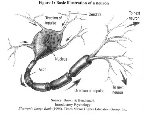
The human brain contains about 10 billion nerve cells, or neurons. The brain's network of neurons forms a massively parallel information processing system. The basic computational unit in the nervous system is the nerve cell or neuron. A neuron has mainly Dendrites (inputs), Nucleus (processing the inputs) and an Axon (output). A neuron receives input from other neurons. Once input exceeds a critical level, the neuron discharges a spike - an electrical pulse that travels from the cell, down the axon, to the next neuron(s). This spiking event is also called depolarization, and is followed by a refractory period, during which the neuron is unable to fire. The axon endings (Output Zone) almost touch the dendrites or cell body of the next neuron. Transmission of an electrical signal from one neuron to the next is effected by neurotransmitters, chemicals which are released from the first neuron and which bind to receptors in the second. This link is called a synapse. Basically, a biological neuron receives inputs from other sources, combines them in some way, performs a generally nonlinear operation on the results, and then outputs the final result. Figure 1 shows a simplified biological neuron and the relationship of its components.

The Basic Artificial Neuron

The first computational neuron was developed in 1943 by the neurophysiologist Warren McCulloch and the logician Walter Pits based on the biological neuron. It uses the step function to fire when threshold µ is exceeded. If the step activation function is used (i.e. the neuron's output is 0 if the input is less than zero, and 1 if the input is greater than or equal to 0) then the neuron acts just like the biological neuron described earlier. Artificial neural networks are comprised of many neurons, interconnected in certain ways to cast them into identifiable topologies as depicted in Figure 2.

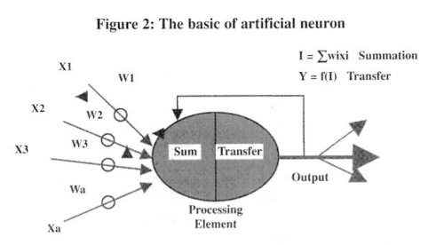
Note that various inputs to the network are represented by the mathematical symbol, x(n). Each of these inputs is multiplied by a connection weights w(n). In the simplest case, these products are simply summed, fed through a transfer function to generate a result, and then output. Even though all artificial neural networks are constructed from this basic building block the fundamentals vary in these building blocks and there are some differences.

Architecture of the Neural Network

Neural nets are a computational framework consisting of massively connected simple processing units. These units have an analog to the neuron in the human brain. One of the most popular neural net paradigms is the feed-forward neural network (FNN) and the associated back-propagation (BP) training algorithm. A brief discussion of both is in order.

Feed-forward networks

In a FNN, the neurons (i.e. the processing units) are arranged in layers i.e. the input, the hidden ones and the output. Feed-forward ANNs allow signals to travel one way—only from input to output. Figure 3 gives a typically fully connected 3- layer feed-forward network topology.

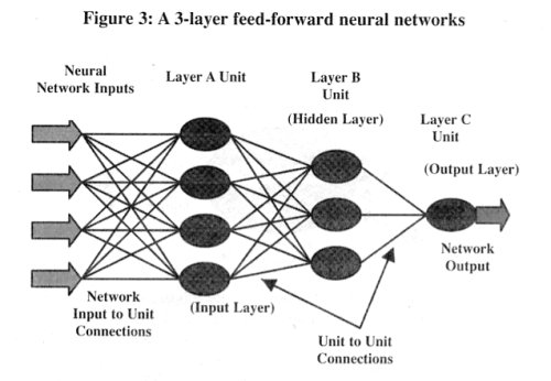
This network has four units in the first layer (layer A) and three units in the second layer (layer B), which are called hidden layers. This network has one unit in the third layer (layer C), which is called the output layer. Finally, this network has four network inputs and one network output. Each networkinput- to-unit and unit-to-unit is modified by a weight. In addition, each unit has an extra input that is assumed to have a constant value of one. The weight that modifies this extra input is called the bias. All data propagate along the connections in the direction from the network inputs to the network output hence the term feed-forward.

Networks layers

The most common type of artificial neural network consists of three groups, or layers, of units: a layer of "input" units is connected to a layer of "hidden" units, which is connected to a layer of "output" units. The activity of the input units represents the raw information that is fed into the network. The activity of each hidden unit is determined by the activities of the input units and the weights on the connections between the input and the hidden units. The behavior of the output units depends on the activity of the hidden units and the weights between the hidden and output units.

Perceptrons

One of the most useful and successful applications of neural networks to data analysis is the multilayer perceptron model (MLP). Multilayer perceptron models are non-linear neural network models that can be used to approximate almost any function with a high degree of accuracy (White, 1992). An MLP contains a hidden layer of neurons that uses non-linear activation functions, such as a logistic function. Figure 4 offers a representation of an MLP with one hidden layer and a single input and output.

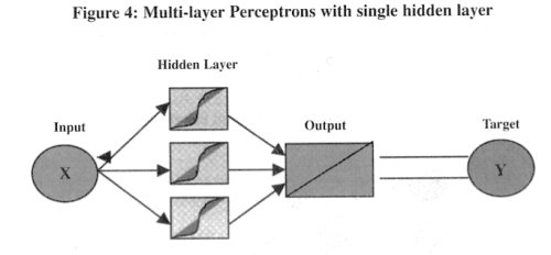
It represents a simple non-linear regression. The number of inputs and outputs in the MLP, as well as the number, can be manipulated to analyze different types of data.

Training Neural Networks

A neural network must be trained before it is actually applied. Training involves feeding the network with data so that it would be able to learn the knowledge among inputs through its learning rule. There are three types of training algorithms: initialization algorithms, supervised learning and unsupervised learning. Initialization algorithms are not really training algorithms at all, but methods to initialize weights prior to training proper. They do not require any training data. In supervised learning, the algorithms alter weights and/or thresholds, using sets of training cases that include both input and target output values. In unsupervised learning, using sets of input training cases, the weights and/or thresholds are altered i.e., output values are not required, and if present are ignored. We use the back-propagation learning algorithm in this paper.

Back-propagation networks

Though several network architectures and training algorithms are available, the back-propagation (BP) algorithm is by far the most popular. The network is considered a feed-forward and the learning is supervised. Multilayer perceptrons neural networks trained by BP consist of several layers of neurons, interconnections, and weights that are assigned to those interconnections. Each neuron contains the weighted sum of its inputs filtered by a sigmoid (S-shaped) transfer function. The error of the output relative to the desired output is propagated backwards through the network in order to adjust the synapse weights.

The learning process of back-propagation neural network is actually an error minimization procedure (Rumelhart, Hinton, and Williams, 1986). A typical BPN model uses three vectors: input vector, one or more hidden vectors, and an output vector. After the input and output vectors are fed into the BPN model, the network first selects parameters randomly and processes the inputs to generate a predicted output vector. After calculating the error between its predicted outputs and the observed outcomes, the network adjusts the parameters in ways that will reduce the error, generates a new output vector; calculates the errors, adjust its parameters again, and so on. The iteration or learning process continues until the network reaches a certain specified error. Figure 5 is a sketch of the stages of a typical BPN model with r inputs, two hidden or intermediate units, and one output unit.

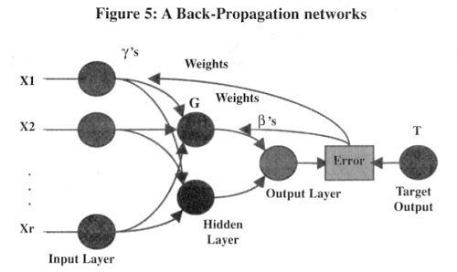
In a general form, the ANN output vector produced by a model or network consisting of r input units, q hidden units, and one output unit can be written as:

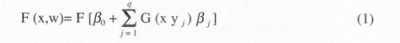
where F(x,w) is the network's final output, F is the activation function for the final step, G is the activation function for a hidden or intermediate unit, X = [1, x1 ,x2..., xr ] is the input vector (including the intercept constant), and w = (γ 1 , γ2,.........., γq, ßj ) is the parameter or weights matrix. Each term γi stands for a (r x 1) vector of weights relating the r input variables to one of the q intermediate units. ßj , refers to a (q x 1) vector of weights relating each intermediate output vector to the final output vector. F and G take the nonlinear sigmoid function.

Neural Networks Model for Time Series Forecasting

Artificial neural network models form an important class of nonlinear models that has attracted considerable attention in many fields of application. The use of these models in applied work is generally motivated by a mathematical result stating that under mild regularity conditions, a relatively simple ANN model is capable of approximating any Borel-measurable function to any given degree of accuracy. Therefore, researchers are trying to use the ANN as a forecasting tool in several time series data. And this paper will focus on the feed-forward neural network technique.

The neural network forecasting model between the output (xt) layer and the inputs (xt-1, xt-2,..... ,xt-p) layer has the following mathematical representation:

where (j = 0; 1; 2; : : : ; q) and ij (i = 0; 1; 2; : : : ; p; j = 1; 2; : : : ; q) are the model parameters often called the connection weights; p is the number of input nodes and q is the number of hidden nodes. The logistic function is often used as the hidden layer transfer function, that is,

Hence, the ANN model of (2) in fact performs a nonlinear functional mapping from the past observations (x_t-1, x_t-2,....., x_t-p; w) to the future value x_t,

where w is a vector of all parameters and f is a function determined by the network structure and connection weights. Thus, the neural network is equivalent to a nonlinear autoregressive model. Note that expression (2) implies one output node in the output layer which is typically used for one-step-ahead forecasting. The simple network given by (2) is surprisingly powerful in that it is able to approximate arbitrary function as the number of hidden nodes q is sufficiently large (Hornik et al., 1990).

As there is no systematic rule and theory in deciding the parameters p and q, simultaneous experiments are often conducted to select an appropriate p as well as q. Once a network structure (p; q) is specified, the network is ready for training-a process of parameter estimation. A back-propagation training system as discussed earlier is used in this study. As in ARIMA model building, the parameters are estimated such that an overall accuracy criterion such as the root mean squared error is minimized. The forecasting performance is measured with the help of two well known criteria:

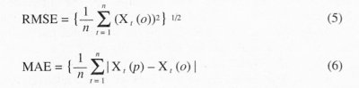
where x(p) and x(o) represent predicted and observed values, respectively.

Empirical Neural Network Model

The objective of the research is to develop a forecasting model capable of predicting the production level of the construction industry in China. In this section, we perform the procedure to establish an ANN model for short-term prediction. Each predicting data is used in the performance validation of an ARIMA and an ANN model. The performance of the model is evaluated by comparing with ARIMA model developed by Dilli and Wang (2002). For the validation and comparison, we have taken a quantitative measure of network performance called "performance index". Root Mean Square Error (RMSE) and Mean Absolute Error (MAE) are used as the criterion of performance index.

Analysis and collection of data

In this paper, the Gross Output Value of Construction Industry and the Gross Domestic Product of the People's Republic of China from 1978 to 2000 are used to study the behavior of production levels of the CI as defined earlier. As mentioned earlier, the contribution of the CI in the overall economic growth of China is significant. At present, China is also in urbanization phase in its overall development. For this reason, the study on the situation and implications of the construction industry to the national economy is vital.

Separation of data into train, verify and test set

Transfer the data into the networks as input

The input data is transformed before the actual modeling takes place. The purpose, according to comp.ai.neural-nets Usenet news W. Sarle (2001), is that standardizing target variables has a more important effect on the initialization of weights than just avoiding saturation. If initialization is poor, local minima will occur. Generally training data in an ANN is scaled for two major reasons. First, input data is usually scaled to give each input equal importance and to prevent premature saturation of sigmoidal activation functions. Secondly, output or target data is scaled if output activation functions have a limited range and the unscaled targets do not match that range. Numeric values have to be scaled into a range that is appropriate for the network. Typically, raw variable values are scaled linearly. We use linear scaling method for obtaining a new range using Statistical Neural Networks (1996), which includes mini/max and mean/SD algorithms that automatically calculate scaling values to transfer numeric values into the desired range.

A simple artificial neural network model

In this section, a neural network model has been developed by applying a real data set under study.

Neural networks architecture

The scheme used in this research consisted of a multilayer perceptron artificial neural network (MLP-ANN), trained with the well-known error backpropagation learning algorithm (Rummelhart et al., 1986), which has been successfully used in a number of macroeconomic forecasting applications as referred above. Following the recommendation of Kuan and White (1994), we use a single hidden layer, since this seems to be appropriate for most economic applications. This is especially true in light of the fact that we have a relatively small sample. Multilayer perceptrons (MLPs) use a linear PSP function (i.e., they perform a weighted sum of their inputs), and a (usually) non-linear activation function. The standard activation function for MLPs is the logistic function, which is used in this paper.

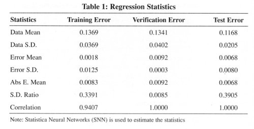
In this analysis, the network consists of single input, hidden and output layer. To determine the appropriate configuration of the feed-forward MLP network several parameters have been varied. The number of neurons in the hidden layer was determined automatically by adapting network complexity. The design procedure was carried out by conducting an extensive search. A maximum of 10 networks were saved balancing the performance against type and complexity (to maintain diversity) by increasing the network set size if the network set is too full. 150 networks were tested and the best 10 networks found were retained by taking account of diversity. The best network found had excellent performance (regression ratio 0.003343, correlation 1.000000, and error 0.000147). The regression statistics for the selected models are shown in Table 1.

Set parameters, values, initialize weights

The parameters and learning algorithms for training the various neural networks used are as follows. Weights: The weights are initialized to a uniformly distributed random value, uniform for all layers with values set at min (0) and max (1). Learning rate (η): The learning rate (0<η<1) is a scaling factor that tells the learning algorithm how much the weights of the connections should be adjusted for a given error. The learning rate η=0.03 is set across presentations. The momentum (α): The momentum parameter (0<α<1) is another number that affects the gradient descent of the weights. The momentum term is added, which keeps the direction of the previous step, thus avoiding the descent into local minima. The momentum term α=0.35 is set across presentations. Epochs: On each epoch, the entire training set is fed through the network, and used to adjust the network weights and thresholds. These parameters decide the forecasting performance of the ANN, however, there is no criterion for deciding optimal parameters. Thus the parameters are decided based on heuristic methods.

Training methodology

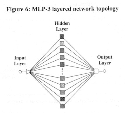
The "cross validation" training methodology is adopted. Training is performed until the error obtained with the testing is reached a minimum. The weighting factors are obtained using the back-propagation algorithm. In the back-propagation methodology a set of initial weights is first chosen at random, after which the network starts the learning process, modifying the weights to reduce the error. The network output is obtained through information sent from the input layer through the hidden layer, facilitated by the activation function. The difference between the predicted value of output and the actual value, called network error, is computed and propagated backwards through the network, layer by layer. The connection strengths are modified in proportion to the error. This process in which the weights are computed is known as an epoch. To avoid over training, the "early stopping" procedure was used by fixing target error = 0 over a number of epochs 100. We trained all of the neural networks for 100 epochs with 16 data points out of 21. The trained neural network models were verified and tested with the remaining 2 data points for each. Among the best retained 10 networks, the network topology: 1:1-31-1:1 Figure 6 is selected as the ANN model because it has the minimum RMSE.

PERFORMANCE EVALUATION

The RMSE and MAE criteria are used to evaluate the accuracy of the outof- sample forecasts. Here, the best performing network with the lowest verification error is a 3 layer multi-percerptron with one hidden layer and 31 hidden nodes network. It has a training error of 0.01217, a verification error of 0.008285 and a test error of 0.007879. This is the root mean square of the errors on each individual case, where the error on each individual case is measured by the network's error function. In this analysis, a comparison of the predicted and the target level is studied with the help of a trained neural network. The forecast obtained is intended to give a vision of the future of the series based on its behavior, given that the actual trends do not change. The plot of the actual and fitted values of the series as depicted in Figure 7 shows that the trend of production levels of CI is increasing steadily implies the strong potential for future growth.

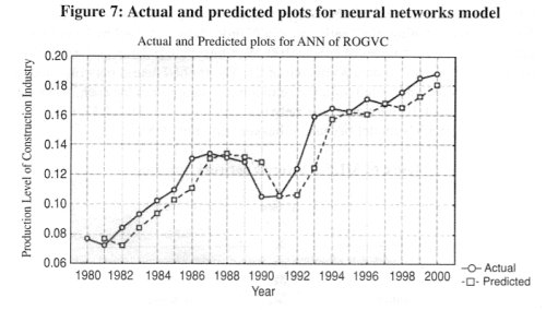
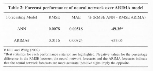
The fitted model is statistically valid as the deviation between the actual and the fitted values is the least. The RMSE and MAE of the best neural network model have reached 0.0078 and 0.00518, respectively. The performance of the empirical ANN model is evaluated by comparing it with the ARIMA model. The result shows that the best neural network model outperforms the ARIMA model by over 49 percent, implying that neural network models can be exploited for noticeable gains in forecast accuracy. This is substantiated by the empirical evidence presented in Table 2.

CONCLUDING REMARKS

The objective of this paper has been to develop an empirical model for the construction industry in China which best fits the data under study and gives a better prediction values with minimum errors so that planner and policy makers can formulate proper policies and programs to promote the industry. Since ANN is one of the non-linear tools that has been in an increasing use to forecast macroeconomic variables, we used this method for our purpose. The novelty of this methodology lies in its ability to capture all indirect relations between variables by introducing hidden layers, and to approximate any non- linearity with the application of the logistic function as activation function. In fact, the literature suggests that ANN can be mathematically shown to be universal function approximations (Hornik et al 1989) and that the neural network outperforms other time-series econometric models such as ARIMA.

The performance of the ANN model has been evaluated by comparing it with the ARIMA model developed by Dilli and Wang (2002). The RMSE and MAE have been used to evaluate the accuracy of the out-of-sample forecasts. Here, the best perform network with the lowest verification error is a 3 layer multi-percerptrons with one hidden layer and 31 hidden nodes network. The results show that the best neural network model outperforms the ARIMA model by over 49 percent, implying that neural network models can be exploited for noticeable gains in forecast accuracy. The gains in forecast accuracy seem to originate from the ability of neural networks to capture asymmetric relationships.

We have used the ANN methodology to forecast the growth of construction industry in China, and have demonstrated its advantages over other traditional time-series methods. However, as it is only a small part of the aggregate economy, other industries and sectors in China need to be studied using the ANN methodology to improve upon forecasting of their behavior. Needless to say, data mining techniques such as the ANN have great potential for improving our understanding of strategic macroeconomic variables that are so crucial in scanning the business environment.

References

Ahmadi H. (1993) Testability of the arbitrage pricing theory by neural networks. In Trippi R.R. and E. Truban, Eds, Neural Networks in Finance and Investing. Probus Publishing

Angstenberger, J. (1996) Prediction of the S&P 500 Index with Neural Networks. In Neural Networks and Their Applications, Chichester, Wiley and Sons, 143-52.

Brown and Benchmark (1995) Introductory Psychology Electronic Image Bank. Times Mirror Higher Education Group Inc.

Bosarge, W. E. (1993) Adaptive Processes to Exploit the Nonlinear Structure of Financial Market. In: R. R. Trippi and E. Turban (eds.): Neural Networks in Finance and Investing. Probus Publishing, 371-402.

Connor, D., (1988) Data Transformation Explains the Basics of Neural Networks. EDN, 138-44.

Dilli and Wang (2002) An application of the ARIMA model for forecasting the production level of construction industry. Journal of Harbin Institute of Technology (New series), vol. 9, sup, 39-45.

Donaldson, R.G., M. Kamstra, and H.Y. Kim (1993) Evaluating Alternative Models for Conditional Stock Volatility: Evidence from International Data. Working Paper, University of British Columbia.

Gonzale, S. (2000) Neural Networks for Macroeconomic Forecasting: A Complementary Approach to Linear Regression Models. Working paper, 07. Department of Finance, Government of Canada.

Hiew, M. and G. Green (1992) Beyond Statistics, A Forecasting System That Learns. The Forum, 5, 1-6.

Hinton, G.E., (1992) How Neural Networks Learn from Experience. Scientific American, 267, 144-51.

Hoptroff, R.G. (1993) The Principles and Practice of Time Series Forecasting and Business Modeling Using Neural Nets. Neural Computing & Applications, 1, 59-66.

Hornik K., Stinchombe M. and White H. (1989) Multi-layer Feed-forward networks are universal approximators. Neural Networks, 2, 359-66.

Hornik K., Stinchombe M. and White H. (1990) Using multi-layer feed-forward networks for universal approximation. Neural Networks, 3, 551-60.

Hutchinson, J. M., T. Poggio, and A.W. Lo (1994) Anonparametric approach to pricing and hedging derivative securities via learning networks. Journal of Finance, 49, 851-889.

Hwarng H. Brian and Ang H.T. (2001) A simple neural network for ARIMA (p; q) time series. Omega, The International Journal of Management Science, 29, 319-33.

Jin, Lu, and Zhang (2002) A regression Model of the Growth Path of Construction Industry. Proceedings of 2002 International Conference on Management Science and Engineering, Moscow, Russia, HIT press, ISBN 7-5603-1793-6/F. 287, Vol.2, 2089-94.

Kamijo, K. and Tanigawa, T. (1990) Stock Price Recognition A Recurrent Neural Net Approach. Proceedings of the International Joint Conference on Neural Networks, 589-621.

Kohzadi, N., M. S. Boyd, I. Kaastra, B. S. Kermanshahi, and D. Scuse (1995) Neural Networks for Forecasting: An Introduction. Canadian Journal of Agricultural Economics, 43, 463-74.

Kuan, C. M. and H. White (1994) Artificial Neural Networks: An Econometric Perspective. Econometric Reviews, 13, 1-91.

Maasumi E., A. Khotanzad, and A. Abaye (1996) Artificial neural networks for some macroeconomic series: a first report. Econometric Reviews, 13 (1), 105-122.

Makridakis, S., A. Anderson, R. Carbone, R. Fildes, M. Hibon, R. Lewandowski, J. Newton, E.Parzen, and R. Winkler (1982) The Accuracy of Extrapolation (Time Series) Methods: Results of a Forecasting Competition. Journal of Forecasting, 1, 111-53.

Mayo, R.E. and Liu G. (1995) Reform agenda of Chinese construction industry. Journal of Construction Engineering and Management, 121(1), 80- 85.

McMenamin Stuart J. (1997) A primer on neural networks for forecasting. Journal of Business Forecasting, 16, 17-22.

Moody John, Levin Uzi and Rehfuss Steve (1993) Predicting the U.S. index of industrial production. Neural Network World, 3(6), 791-94.

Moody, J. (1995) Economic Forecasting: Challenges and Neural Network Solutions. Keynote talk presented at the International Symposium on Artificial Neural Networks, Hsinchu, Taiwan.

National Bureau of Statistics (2001), China Statistical Year Book. China Statistics press, Beijing.

Prudence S. (2002) Monetary Conditions & Core Inflation: An Application of Neural Networks. Working paper, Research Services Department, Research and Economic Programming Division, Bank of Jamaica.

Rumelhart, D.E., G.E. Hinton, R.J. Williams (1986) Learning Internal Representations by Error propagation. Parallel Distributed Processing, D.E. Rumelhart, J.L. McClelland (Eds.), MIT Press, Cambridge, MA, Volume 1, 318-62.

Sharda, R. and R. Patil (1990) Neural Networks as Forecasting Experts: An Empirical Test. Proceedings of the 1990 International Joint Conference on Neural Networks Meeting, Vol. 2, 491-94.

Sharda, R. and R. Patil (1992) Connectionist Approach to Time Series Prediction: An Empirical Test. Journal of Intelligent Manufacturing, 3, 317-23.

Swanson, N. R. and H. White (1995) A model selection approach to assessing the information in the term structure using linear models and artificial neural networks, Journal of Business and Economic Statistics 13, 265-75.

Swanson, N.R., and White, H. (1997a) A model selection approach to real time macroeconomic forecasting using linear models and artificial neural networks. Review of Economics and Statistics, 79, 540-50.

Swanson, N.R., and White, H. (1997b) Forecasting economic time series using adaptive versus non-adaptive and linear versus nonlinear econometric models. International Journal of Forecasting, 13, 439-61.

Statistica Neural Networks (1996) Trajan Software Ltd. StatSoft Inc. 2300 East 14th Street, Tulsa, OK 74104, USA.

Tang, Z., C. de Almeida, and P. Fishwick (1991) Time Series Forecasting Using Neural Networks vs. Box-Jenkins Methodology. Simulation,. 57, 303-10.

Tkacz, G. (1999) Neural Network Forecasts of Canadian GDP Growth Using Financial Variables. Mimeo, Bank of Canada.

Tkacz, G. (2001) Neural network forecasting of Canadian GDP growth. International Journal of Forecasting, 17, 57-69.

Tkacz, G. and Hu, S. (1999) Forecasting GDP Growth Using Artificial Neural Networks. Working Paper, Bank of Canada, 99-3

W. Sarle (2001) Comp.ai.neural-nets. Usenet news FAQ, http://www.faqs.org/faqs/ai-faq/neural-nets/.

Walczak, S. (2001) An Empirical Analysis of Data Requirements for Financial Forecasting with Neural Networks. Journal of Management Information Systems, Spring, 17, (4), 203-22.

Wasserman P.D. (1989) Neural Computing: Theory and Practice. Van Nostrand Reinhold, New York.

White, H (1988) Economic Prediction using Neural Networks: The Case of IBM Daily Stock Returns. Proceeding of the IEEE International Conference on Neural Networks II, 451-58.

White, H. (1992) Artificial Neural Networks: Approximation and Learning Theory, Cambridge and Oxford, Blackwell.

Widrow, B. and Sterns D. (1985) Adaptive Signal Processing, Englewood Cliffs. NJ, Prentice-Hall.

Wong, F. S. (1990) Time Series Forecasting using Back-propagation neural Networks. Neurocomputing, 2, 147-59.

Xu, K., Xie, M., Tang, L.C. and Ho, S.L. (2003) Application of neural networks in forecasting engine systems reliability. Applied Soft Computing, 2, 255- 68.

Yoon, Y. and G. Swales (1990) Predicting Stock Price Performance. Proceeding of the 24th Hawaii International Conference on System Sciences, 4, 156- 62.

Zhang, G., Patuwo E.B. and Hu, M.Y (1998) Forecasting with artificial neural networks: the state of the art. International Journal of Forecasting , 14, 35-62.