Vol. 16 No. 2 January 2005
A Transportation-Scheduling System for Managing Silvicultural Projects
Jorge F. Valenzuela
H. Hakan Balci
Timothy McDonald
Auburn University
Alabama, USA
ABSTRACT
A silvicultural project encompasses tasks such as site-level planning, regeneration, harvest, and stand-tending treatments. An essential problem in managing silvicultural projects is to efficiently schedule the operations while considering project task due dates and costs of moving scarce resources to specific job locations. Transportation costs represent a significant portion of the total operating cost. The main difficulty in developing such a management system is finding an optimal transport schedule while handling complicated constraints, such as precedence and temporal relations among project tasks, project due dates, truck routing, weather, and other operational conditions. It is well known that finding an optimal solution to these types of problems involves high computational complexity. They are usually NP-hard. For this reason, we propose to use simulated annealing -a meta-heuristic optimization method- that interacts with a network simulation model of the system in which the precedence and temporal relations among project tasks and logistics are explicitly accounted for. The approach has been tested using data provided by a silvicultural contractor located in Alabama. The results obtained solving one instance of a small size problem with five worksites showed that the best solution could be found in less than four minutes using a personal computer with a processor Pentium III (1 GHz). A good solution for a larger problem with twenty worksites was found in thirty minutes. Also a resource analysis is performed to evaluate the impact of each resource on the best solution.
Keywords: Project management, silvicultural systems, forest operations, meta-heuristic, optimization, simulation.
INTRODUCTION
Silviculture is defined as managing forest vegetation by controlling stand establishment, growth, composition, quality and structure for the full range of forest resource objectives [7]. This is a broad definition encompassing a multitude of concepts, all of which must be translated into manipulations of a given trait or characteristics to effect some change at a stand or sub-stand. The range of manipulations used on any given stand can vary considerably, but as the science of silviculture matures the complexity and number of entries into stands for management activities has tended to increase. At the same time, the need to reduce the cost of these activities has lead to specialized equipment and contractors to implement custom prescriptions efficiently across many locations. When the primary resource being manipulated is timber, cost of silvicultural operations is of particular importance and new ways are being sought to reduce the amount of input resources needed to establish and maintain maximum growth rate.
Forest landowners in the Southeast US, particularly large industrial forest product companies, often use silvicultural service providers as a means of implementing their management prescriptions. These providers can perform a broad spectrum of management activities at low cost, but, as in logging, there is always a need to further improve the efficiency of the operations. Service providers have turned to new technology in order to improve their cost effectiveness, in particular adapting techniques from precision agriculture to reduce chemical inputs. Adopting logistical strategies used successfully in other industries also holds the promise of improving operational efficiency. Providing silvicultural services typically implies performing numerous operations simultaneously across a large geographic area. These operations share equipment resources. For example, a crawler tractor might be used for road improvement work as well as in site preparation plowing. Scheduling the use of these limited resources has a large impact on the efficiency of the entire operation. Equipment must be dispatched to sites in a sequence that minimizes total moving costs, primarily a function of distance traveled, and that also accounts for temporal aspects of task completion. The scheduling process is further complicated by constraints on movement of the equipment and by external factors such as weather. Management and scheduling of these activities is currently done by people with experience in such matters, but as companies become larger and the number and complexity of jobs increases, silvicultural service providers are looking for improved methods of assigning resources to jobs in a manner that optimizes their operational efficiency.
The scope of scheduling silvicultural tasks lies within what is called project scheduling under resource constraints, which has been extensively studied [6]. One of the simplest project scheduling approaches is the Critical Path Method (CPM) [17]. In this method, the set of tasks are represented as a network to denote the precedence relations among pairs of tasks. The goal in the CPM approach is to determine the smallest possible project completion time without violating the precedence relations of the tasks. The method assumes infinite availability of resources. A more realistic variant of the CPM is the Resource-Constrained Project Scheduling problem (RCPSP) [10]. Several approaches have been proposed to solve the RCPSP. Pritsker et al. [15] proposed one of the first mathematical formulations, a 0-1 linear programming model to solve the RCPSP. The formulation requires the definition of up to nT binary variables, where n is the number of activities and T is the number of time periods. The complexity of the model is O(n2+mT), where m is the number of resources. More 0-1 linear programming models can be found in [3, 11]. Although the RCPSP is more realistic, it still has some limitations. One of the drawbacks of the RCPSP formulation is that it assumes constant availabilities of the resources during the planning horizon, but it is common in practice that machines are scheduled for maintenance or they are required for other projects. Also, due dates cannot be considered within the RCPSP framework. The Generalized Resource-Constrained Project Scheduling Problem (GRCSP) [10] overcomes some of these limitations and has been successfully used in manufacturing applications [4]. Despite its high practical relevance, the GRCSP is still not a good model for use in scheduling silvicultural tasks since the method neglects transportation costs. There is also a large literature on transportation routing problems, which are modeled and solved with various approaches [8, 12]. The reader is referred to [5] for an overview of vehicle routing problems. However, these models do not implicitly account for the ordered sequence of tasks that may use these transportation resources.
This paper proposes a computer meta-heuristic model for scheduling simultaneously several silvicultural projects, each project consisting of an ordered sequence of tasks requiring the use of limited equipment resources. The model implicitly considers due dates of each project, the order and nature of steps to complete tasks, task-duration times, resource requirement constraints, task-precedence relationships, geographic location of the projects, transportation costs, and due date violation costs. The goal of the model is to allocate shared expensive assets and minimize transportation costs and completion time of the projects. The resulting optimization problem is a nontrivial generalization of the GRCSP. To solve meaningful problems, we have developed an optimization procedure consisting of a simulated annealing (SA) [16] algorithm that interacts with a network simulation model of the silvicultural multi-project system.
The paper has been organized as follows. In section 2, we describe the proposed approach. In section 3, we describe our experimental methodology and summarize numerical and performance results. In section 4, a resource capacity sensitivity analysis is performed to evaluate the impact of each resource on the best scheduling solution.
PROPOSED APPROACH
The problem of managing silvicultural projects can be formulated as efficiently scheduling transportation and project tasks while considering project due dates and costs of moving resources to specific job locations. Scheduling transport among several competing locations and functions is critical in efficiently managing silvicultural projects. Transportation costs represent a significant portion of the total operating cost. Trucks are needed for delivering timber to mills and for carrying machinery between worksites, which can be located anywhere within a large geographic area. A transportation management system that allocates limited truck resources optimally among competing interests and takes into account project due dates could increase the total operational efficiency of a procurement entity.
Problem Description
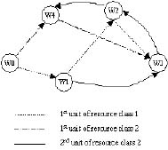
A solution X to the transportation-scheduling problem consists of a set of routes for each of the resources that visit each project location such that all projects can be completed. A route specifies the sequence in which the resource will visit the worksites. For example, for a set of projects consisting of four worksites and three resource units, a solution could be given by the set of routes X= {(1, 4, 3, 2, 3), (2,1,4), (4,2,1)}. In this solution, resource 1 is scheduled to start at worksite 1, then travel to worksite 4, and so on. In our formulation, we assume R different classes of resources and that each class k (k=1,..,R) has rk identical units available. For example, four similar tractors (three John Deere and one Allis Chalmers) may form the "resource class" tractor. Each tractor is then a resource unit. We assume that once an activity releases a particular resource, the resource can start its travel to the next activity scheduled to use this resource unit. The next activity can be located at the same or at a remote worksite. This assumption implies that if the resource unit requires a truck, the truck will be available to transport it. Notice, however, that a truck can also be modeled as a resource unit and it can be requested by activities. In the case that the resource unit has its own transportation (can move by itself), the assumption is also valid. Figure 1 shows an example of a transport schedule (a solution) for a forest project with 5 worksites, two identical units of the resource class 1, and one unit of resource class 2. Here, worksite 0 (W0) is assumed to be a central worksite where maintenance activities can be performed. The figure shows that the first unit of resource class 2 is currently at worksite 0 and is scheduled to visit worksite 4 and then worksite 3.
Figure 1. A solution for a multi-project problem.
Mathematical Model
We assume that the silvicultural multi-project consists of N spatially dispersed worksites. Each worksite is considered one project. The quantity dij is the distance between worksites i and j. At each worksite i (i=0, ...,N-1), a set of Mi tasks need to be performed. The set of tasks to be performed at worksite i is denoted by {t1i, t2i,…}. The task precedence relationships, resource requirements, and execution times of the tasks are all part of a project description, which we denote by W=W0,..,Wi ,..,WN-1]. The due dates of the projects are denoted by D=[D0,..,Di,..,DN -1]. Figure 2 presents a hypothetical example of a project description outlining the tasks to be performed at worksite 1, project description W1. The figure shows the precedence relationships, duration, and resource requirement of each activity. The available resource classes, quantities, and initial positions of each of the resource units are part of the transport description, which we denote by T = [T1,…,Tj,..., TR] (R resource classes.)
The mathematical model for minimizing project durations can be written as follows:
Min z
Subject to C =
F(X; W,T); C
£ 1z; C £ D
Where C is a vector in which entry i is the completion time of project i. F(.) is a function that evaluates the completion time of each project given the descriptions of the projects and transport, and the solution X. The vector 1 denotes a vector with all entries equal to 1, i.e. 1=[1, 1,…,1].
Solution Approach
The solution approach consists of two main components, a network simulation model and a search heuristic. The simulation model is used to evaluate the function F, i.e. the completion time of the projects. The purpose of the search heuristic component is to select a good solution X, and is implemented using a Simulated Annealing (SA) algorithm. In the literature there are multiple applications of SA to forest management and planning. Öhman and Lämås [14] studied long-term planning of harvest activities considering biodiversity, recreation and new road planning. They concluded that the spatial dimension of the problem increased complexity, but that the SA approach could effectively generate optimal solutions. In another study [1], Baskent and Jordan used the SA approach to solve a new landscape management model. They tested their model on a 20,000 ha (987 stands) hypothetical test problem. The result showed that the SA meta-heuristic technique was capable of solving large-size stochastic problems with hard constraints.
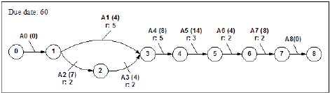
Figure 2. Description of worksite/project W1*
The SA algorithm starts by generating an initial solution to the transportation-scheduling problem. In our approach, the initial solution can be either provided by the user or generated randomly. The simulation model is next used to evaluate the quality of this initial solution. The inputs to the simulation model are the data corresponding to the project descriptions and the transport sched ule for the resources (a solution). The simulation model outputs performance measures, such as completion times for the tasks and distances traveled by the resources. The SA algorithm searches for a better solution using the information provided by the simulation model and the current solution. We have implemented three neighbor operators to perturb the current solution. One operator generates a new solution by switching two worksites (randomly selected) of the current solution within a route of a specific unit. The second operator generates a new solution by switching two worksites between two different units of a same class. The units and the worksites are randomly selected. The third operator generates a new solution by moving one worksite from a unit to another unit of the same resource class. We use a random selection process to choose the operator to be applied at each neighborhood search. The search procedure uses the simulator every time that it needs to evaluate the performance of a new solution. An optimal or close to optimal solution is obtained by iteratively running this search procedure. Figure 3 shows a block diagram of the solution approach.
Simulated Annealing
Simulated Annealing [16] is one of the nature-inspired heuristics that are applied to combinatorial optimization problems. It was derived from statistical mechanics. The algorithm, which was proposed by Kirkpatrick et al. [9], is based on an analogy between annealing treatment of solids and solving combinatorial optimization problems. Annealing is the physical process of heating a solid and then cooling it down slowly until it crystallizes. At a given temperature, the probability distribution of system energies is determined by the Boltzmann's probability equation:
P(E)=αe[-E/kT] (1)
where E is system energy, k is Boltzmann's constant, T is the temperature and P(E) is the probability that the system is in a state with energy E. To simulate the evolution to thermal equilibrium of a solid for a fixed value of temperature T, Metropolis et al. [13] proposed a Monte Carlo method, which generates sequences of the states of the solid.
In the analogy between solving a combinatorial optimization problem and the annealing process, the states of the solid represent the feasible solutions of the optimization problem. The energies of the states correspond to the values of the objective function computed for those solutions. The minimum energy state corresponds to the optimal solution of the problem and rapid quenching can be viewed as local optimization. The basic steps of a SA algorithm are as follows:
Step 0: Create an initial solution. This is the first current solution.
Decide the initial temperature, number of repetitions at each temperature step, temperature reduction rule and total number of iterations to be performed.
Step 1: Generate a new set of solution/s from the current solution.
Step 2: Evaluate the solution in terms of the objective function. Keep track of the best solution found so far.
Step 3: If the newly created solution is better, then update the current solution to the newly found better solution. If not, decide whether the new solution can still become the current solution, depending on Metropolis's criterion [13]. If it passes the criterion, then the newly found solution becomes the current solution; otherwise the current solution stays the same.
Step 4: Iterate through steps 1, 2 and 3 for a defined number of times as decided by the number of repetitions at each temperature step. After those many repetitions go to Step 5.
Step 5: Decrease the temperature using the decided reduction criterion. Iterate through steps 1, 2, 3 and 4 for the decided number of times. After those many number of iterations, stop. Use the best solution found so far.

Figure 3. Optimization Model.
EXPERIMENTAL RESULTS
Using data from a silviculture contractor located in South Alabama, we have created a test-bed problem to verify our approach. The problem consists of four projects that are performed at four different sites and one central site, namely worksite 0. Table 1 gives the distances between each of the worksites.
Table 1. Distance between worksites (in miles).
| Worksites | 0 | 1 | 2 | 3 | 4 |
| 0 | - | 107.5 | 220 | 330 | 82.5 |
| 1 | - | 112.5 | 437.5 | 142.5 | |
| 2 | - | 550 | 245 | ||
| 3 | - | 322.5 | |||
| 4 | - | ||||
The set of tasks performed at each of the worksites are given in Table 2. This table describes location (worksite), duration, precedence, and classes of moveable resource for each task.
Table 2. Task description.
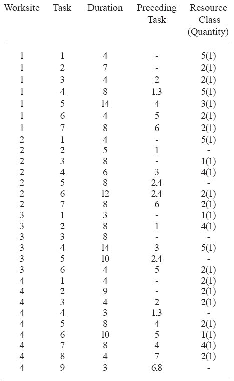
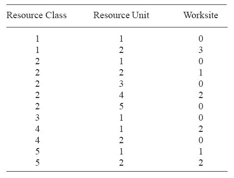
We assume five classes of moveable resources are available. These resources are considered critical for the operation of the projects. Table 3 gives the number of identical units and their initial locations for each resource class. We assume that the resources move at a fixed average speed of 50 mph. Notice that this assumption is not a restriction since each moving object in the simulation can be modeled to move at its own speed.
Table 3. Resource units and their initial positions.
Minimizing Project Durations (Makespan)
In order to test our model, we first set the objective of the optimization model as minimizing the makespan of all the projects. The makespan of a project is defined as the completion time of the last task. Minimizing project durations is equivalent to maximizing the utilization of the resources. After running the algorithm several times with different parameters, we decided to set up the initial and cooling temperature of the SA algorithm to be 150 and 10 F°, respectively. In addition, the temperature of the SA algorithm is decreased at each iteration by 2%. At each temperature step, the neighborhood of the current solution is searched two hundred times. To evaluate the sensitivity of the SA algorithm to the initial solution, we ran the algorithm ten times. For each run the initial solution was randomly generated. The results of the test problem - best, average, and worst - of ten replications were 225, 231 and 253 hours, respectively.
To find whether the best solution was optimal, we computed the objective function assuming an infinite number of resource units available. In this relaxed problem, all projects can be independently completed at a minimum time, determined by the precedence relationships only, and not by the availability of the resources. The minimum makespan of this problem can be easily calculated by hand and it was equal to the minimum makespan of our best solution to the original problem. Therefore, we concluded that the best solution was optimal. However, if they had not been equal, then we could not conclude that the best solution was optimal. Nevertheless, the solution of the relaxed problem could be used as a lower bound.
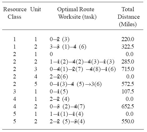
The best solution, for this particular case, which was also solution, the total distance traveled by the resources was 3423 miles. As shown in table 4, the 2nd unit of resource class 1 had a route defined as "3®3 (1)®4 (6)", meaning the initial location of this unit was worksite 3 and it was scheduled to subsequently be used by the 1st task at the same worksite and by the 6th task at worksite 4. This particular route was 322.5 miles long.
Table 4. Routes that minimized project durations.
Minimizing Total Traveled Distance
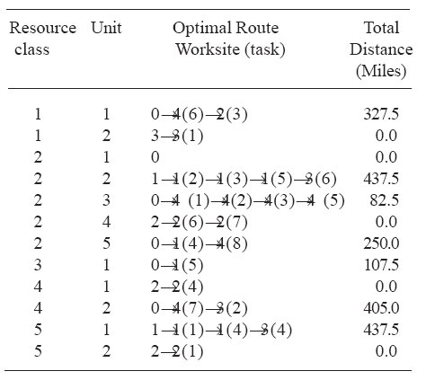
Next, we changed the objective function to minimize the total traveled distance. The results - best, average, and worst - of the computational experiment were 2047.5, 2387.5, and 2717.5 miles, respectively. The best solution is illustrated in Table 5. For this solution the duration of the longest project is 366.55 hours.
Table 5. Best routes that minimize the total traveled distance.
It is clear that the real-world `optimal' solution would require making an explicit trade-off between the objective of minimizing the makespan and minimizing the total traveled miles. Figure 4 depicts this trade-off by displaying a set of feasible solutions. Each point identifies the makespan and traveled miles of a particular solution.
Notice that the three points joined by the line dominate all other solutions. All solutions lying on this line are called Pareto optimal solutions [2]. Pareto optimality is a measure of efficiency. A solution is Pareto optimal if there is no other solution that makes every objective better off. A final decision that explicitly considers the trade-off between the makespan and the traveled miles should lie on or near this Pareto curve. Notice also that the range of the solutions is quite large. For example, there are many solutions that have the minimal makespan of 225 hours, but have different total traveled miles ranging from 2410 to 3400 miles. Here, there is a potential for an improvement of 990 fewer miles. Furthermore, without an optimization procedure, the company could be operating at any point to the right of the line in the figure, for example the point marked `A' where traveled total distance is 2750 miles and makespan is 325 hours. By using one of the solutions lying on the curve, say traveled total distance equal to 2300 miles and makespan equal to 260 (point marked `B' in the figure), the company could reduce the completion time by 65 hours (20%), and the total traveled distance by 450 miles (16%).
Minimizing Project Durations and Total Traveled Miles
The trade-off of makespan and total traveled miles was modeled using a linear cost function. We added a penalty cost of K1 dollars per each hour that a project was overdue and a cost of K2 dollars per each hour spent traveling between sites. We assumed equal overdue penalty costs for all the projects for simplicity only. Introducing different penalty costs for each of the projects can been done in a straightforward manner. The number of overdue hours for each project was calculated in hours as:
Overdue hours = MAX (0, project completion hours - due date hours) (2)
In equation 2, the term "due date" refers to the number of hours from the current hour in which the project is required to be completed. The total overdue hours for all worksites was computed by adding up the individual overdue hours. Thus, the total cost of a particular schedule-solution was the sum of the total overdue penalty costs and total travel time costs:
Total Cost = K1 x Total Overdue Hours + K2 x Total Travel Time Hours (3)
In our example, we assumed that K1 and K2 are 50$/hour and 80$/hour, respectively. Moreover, we assumed for this example that the due dates of each project were 225, 196, 180, and 187 hours. After running the solution algorithm, the best scheduling solution was found to have a total cost of $4,381. This schedule completed all the projects on time (before due date) and had a total traveled distance of 2,738 miles.
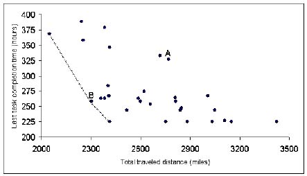
Figure 4. Trade-off between makespan and traveled miles.
In Table 6, we have summarized the total costs by minimizing each cost component separately and both costs simultaneously. If we set the objective to minimize the total overdue hours of the projects only, the overdue cost is zero, but the travel cost is $4,249. On the other hand, if we set the objective to minimize just the total travel hours, the travel cost is $3,246 and the overdue cost is $46,092. However, if we set the objective to minimize both total overdue hours and the total travel hours, the proposed algorithm gives a solution in which the travel costs is $4,381 and zero overdue cost. All projects are completed on time.
Table 6. Cost components with different objectives.
| Objective | Travel cost ($) | Overdue cost ($) | Total cost ($) |
|---|---|---|---|
| Minimizing total overdue hours | 4,249 | 0 | 4,249 |
| Minimizing travel time | 3,246 | 46,092 | 49,338 |
| Min. both total overdue and travel time | 4,381 | 0 | 4,381 |
Sensitivity Analysis
The previous results depended on the values of K1 and K2. To observe the effect of these two cost coefficients, we changed K1 within the range $10/hour to $70/hour and K2 within the range $40/hour to $100/hour. Table 7 gives the cost components, travel miles and overdue hours for different values of K1 and K2.
Table 7. Total cost of best solution when travel and due-date costs are minimized
| K1 ($/hour) | K2 ($/hour) | Total Cost ($) | Overdue Cost (% of total cost) | Travel Cost (% of total cost) | Traveled mile |
|---|---|---|---|---|---|
| 10 | 40 | 2374 | 8% | 92% | 54.43 |
| 10 | 60 | 3635 | 16% | 84% | 50.89 |
| 10 | 80 | 4667 | 11% | 89% | 51.98 |
| 10 | 100 | 5491 | 12% | 88% | 48.53 |
| 30 | 40 | 2326 | 0% | 100% | 58.16 |
| 30 | 60 | 3752 | 0% | 100% | 62.54 |
| 30 | 80 | 4419 | 0% | 100% | 55.24 |
| 30 | 100 | 6203 | 0% | 100% | 62.03 |
| 40 | 40 | 2326 | 0% | 100% | 58.16 |
| 40 | 60 | 3490 | 0% | 100% | 58.16 |
| 40 | 80 | 5003 | 0% | 100% | 62.54 |
| 40 | 100 | 5524 | 0% | 100% | 55.24 |
| 50 | 40 | 2326 | 0% | 100% | 58.16 |
| 50 | 60 | 3490 | 0% | 100% | 58.16 |
| 50 | 80 | 4381 | 0% | 100% | 54.76 |
| 50 | 100 | 6254 | 0% | 100% | 62.54 |
| 60 | 40 | 2104 | 0% | 100% | 52.59 |
| 60 | 60 | 3490 | 0% | 100% | 58.16 |
| 60 | 80 | 4653 | 0% | 100% | 58.16 |
| 60 | 100 | 5476 | 0% | 100% | 54.76 |
| 70 | 40 | 2187 | 0% | 100% | 54.67 |
| 70 | 60 | 3490 | 0% | 100% | 58.16 |
| 70 | 80 | 4653 | 0% | 100% | 58.16 |
| 70 | 100 | 5816 | 0% | 100% | 58.16 |
To study the effect of the problem size on the CPU time, we ran the algorithm with four larger problems. These new problems had 8, 10, 15, and 20 worksites. We set the size of the local search proportional (40 times) to the number of worksites. Figure 5 shows the CPU time versus the number of worksites of each of these problems for the cases in which the local search was kept constant over the problem size, and when the local search was proportional to the problem size.
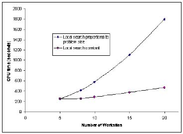
Figure 5. CPU time versus problem size (Pentium III 1 FHz and 256 MB)
RESOURCE CAPACITY PLANNING
Resource capacity planning is the process of determining how much equipment is required to accomplish tasks. The goal of capacity planning is to achieve a balance between resource capacity and work demand. Resource capacity planning is critical in the current forest business environment as companies strive to achieve the highest return on investment for their project portfolios while minimizing expenses. Project-related work often requires significant adjustment during its lifecycle to align capacity and demand. Such changes inevitably affect other work. Our proposed model can also be used to assess the impact of changes on the amount of equipment. The ability of the model to manage capacity is achieved by making modifications to the number of resources and observing the performance of the projects. The performance of the projects is evaluated by the total cost. Figure 6 shows the percent reduction in total cost when a new resource is added and the added resource starts at worksite 0. For example, adding one unit of resource 1 the total cost of completing all the projects can be reduced by 13%. This is from $4,381 to $3,812. Similarly, if one unit of resource 2, instead of resource 1, is added the total cost of completing all the projects can be reduced by 4%. The capacity analysis shows that for this example addition of resources 1 and 5 provide the highest cost reductions.
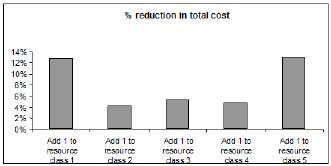
Figure 6. Capacity analysis by increasing the number of resources.
We next decrease each resource class in one unit. Figure 7 shows the percent of increase in total cost when one unit of each resource is removed. For example, removing one unit of resource 1 the total cost of completing all the projects can be increased by 13%. This is from $4,381 to $4,942. Similarly, if one unit of resource 2, instead of resource 1, is removed then the total cost of completing all the projects can increase 20%, i.e. to $5,278. Notice that resources 4 and 5 have the highest cost increases, 43% and 61%, respectively. Reduction in resource class 3 is not shown in Figure 7, because resource class 3 has only one unit that the reduction leads to an infeasible solution.
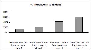
Figure 7. Percent increase in total cost when one unit of a resource class is removed.
DISCUSSION
A heuristic procedure for scheduling transport resources to tasks at remote locations has been described. The use of a simulation model makes the proposed approach very attractive because detailed features of a company's operation can be easily included. The results obtained solving one instance of a small size problem showed that the best solution could be found in less than four minutes using a personal computer with a processor Pentium III (1 GHz). Notice that the problem may be small compared with a real world problem, but the search space of the problem is still quite large. For example, the number of all possible paths, through which a particular resource unit can visit worksites is a function of the number of permutations of all these locations. Considering that the small size problem has 12 resources and that each resource unit visits on the average 4 locations, the size of the solution space is roughly (4!)12, which is close to 1017.
The results from problems of larger sizes show that the relation between CPU time and number of worksites depends strongly on the size of the local search. If the number of local searches is set independently of the problem size (number of worksites), the relation between CPU time and problem size is almost linear; however, when the number of local searches is set proportional to the number of worksites, the relation between CPU time and problem size becomes close to a quadratic function. The CPU time depends more on the size of the local search than on the execution time of the simulator. Nevertheless, if a real world problem is too big to be solved directly with our approach, the problem can be partitioned into smaller manageable sub-problems by identifying resources and geographic areas for each of them and using the proposed algorithm solve each sub-problem separately.
A silvicultural services company could achieve significant savings by using this approach to schedule its operations. It is well known that transportation costs represent a significant portion of the total operating cost of a forest products company. Additionally, transportation cost reduction has positive environmental effects as fuel use is minimized. Future research plans are to incorporate into the simulation model random components such as breakdowns of machines or trucks and weather uncertainties.
ACKNOWLEDGEMENT
This research was supported by the USDA Forest Service Forest Operations Research Unit.
AUTHOR CONTACT
Professor Valenzuela can be reached by email at --
jvalenz@eng.auburn.edu
REFERENCES
[1] Baskent, E.Z., and G.A. Jordan. 2002. Forest landscape management modeling using simulated annealing. Forest Ecology and Management. 165(1-3): 29-45.
[2] Caballero, R., T. Gomez, M. Luque, F. Miguel, and F. Ruiz. 2002. Hierarchical generation of pareto optimal solutions in large-scale multiobjective systems. J. of Computers & Operations Research. 29: 1537-1558.
[3] Demeulemeester, E., and W. Herroelen. 1997. A branch-and-bound procedure for the generalized resource-constrained project scheduling problem. Operations Research. 45: 201-212.
[4] Demeulemeester, E., and W. Herroelen. 1996. Modeling setup times, process batches and transfer batches using activity network logic. European J. of Operational Research. 89: 355-365.
[5] Desrosiers, J., Y. Dumas, M.M. Solomon, and F. Soumis. 1995. Time constrained routing and scheduling. In M.O. Ball, T.L. Magnanti, C.L. Monma, and G.L. Nemhauser, editors, Network Routing, Handbooks in Operations Research and Management Science, 8: 35-139.
[6] Gordon, J. and R. Tulip. 1997. Resource scheduling. Int. J. of Project Management. 15(6): 359-370.
[7] Helms, J. 1998. The Dictionary of Forestry. Society of American Foresters, Bethesda, MD, USA.
[8] Jansen, B., P.C.J. Swinkels, G.J.A. Teeuwen, B.A. Fluiter, and H.A. Fleuren. 2004. Operational planning of a large-scale multi-modal transportation system. European J. of Operational Research. 156: 41-53.
[9] Kirkpatrick, S., C.D. Jr. Gelatt, M.P. Vecchi. 1983. Optimization by simulated annealing. Science. 220: 671-680.
[10] Klein, R. 1999. Scheduling of resource-constrained projects. Kluwer Academic Publishers, Boston, 392 p.
[11] Kolish, R. 1995. Project scheduling under resource constraints: Efficient heuristics for several problem classes (production and logistics). Springer-Verlag, Heidelberg, 212 p.
[12] Liu, S.T., and C. Kao. 2004. Solving fuzzy transportation problems based on extension principle. European J. of Operational Research. 153: 661-674.
[13] Metropolis, N., A. Rosenbluth, M. Rosenbluth, A. Teller, and E. Teller. 1953. Equation of state calculations by fast computing machines. J. of Chemical Physics. 21: 1087-1092.
[14] Öhman, K., T. Lämås. 2003. Clustering of harvest activities in multi-objective long-term forest planning. Forest Ecology and Management. 176(1-3): 161-171.
[15] Pritsker, A., L. Watters, and P. Wolfe. 1969. Multiproject scheduling with limited resources: A zero-one programming approach. Management Science. 16: 93-108.
[16] Vidal, R.V.V. 1993. Applied Simulated Annealing. Springer-Verlag, Berlin, 396 p.
[17] Winston, W. 2004. Operations research: Applications and algorithms. Duxbury Press, Toronto, 1418 p.
The author are, respectively, Assistant Professor, and PhD Student in the Department of Industrial and Systems Engineering, and Associate Professor, Department of Biosystems Engineering, Auburn University.