Vol. 16, No. 2 July 2005
Kazuhiro Aruga
Utsunomiya University
Tochigi, Japan
John Sessions
Oregon State University
Oregon, USA
Abdullah Akay
Kahramanmaras Sutcu Imam University
Kahramanmaras, Turkey
Woodam Chung
The University of Montana
Montana, USA
The authors are, respectively, Associate Professor, Department of Forest Science, Utsunomiya University; Professor, Department of Forest Engineering, Oregon State University; Assistant Professor, Forest Engineering Department, Kahramanmaras Sutcu Imam University; and Assistant Professor, School of Forestry, The University of Montana.
ABSTRACT
We developed a forest road design model that simultaneously optimizes horizontal and vertical alignments of forest roads using a high resolution Digital Elevation Model (DEM). Once an initial horizontal alignment is established by locating a series of intersection points, the model generates alternative horizontal and vertical alignments and cross sections along the road prism. The model also estimates earthwork volume and construction and maintenance costs for given road alignments and their spatial locations. The model then optimizes road alignments based on construction and maintenance costs using Tabu Search, one of the modern heuristic techniques.
The model was applied to a part of Capitol Forest in Washington State, USA, where a high resolution DEM derived from LiDAR (Light Detection and Ranging) data was available. First, the program generated an initial horizontal alignment with the length of 827m and five horizontal curves based on manually selected intersection points. Then, the vertical alignment was optimized based on the initial horizontal alignment, which resulted in a total cost of $50,814, considering construction and maintenance costs. The optimized forest road alignment, whose horizontal and vertical alignments were simultaneously optimized during the search process, reduced the total cost and the road length by 36% and 19% compared to the initial horizontal alignment, respectively.
Keywords: Forest road alignment, Forest road design, Heuristic optimization technique, High resolution DEM, Tabu Search, Washington State.
INTRODUCTION
In forest road design, it is a difficult task for a forest engineer to find a good alignment from a large number of alternatives considering social, economic and environmental impacts. Since the number of alternatives connecting two end points is unlimited, a manual design may reach neither an optimal design nor a near-optimal design. Forest road design programs have been developed in order to reduce workloads for forest engineers in drawing a forest road plane, a forest road profile, a large number of cross sections, and in calculating earthwork volumes. To reach the best alignment alternative subject to all the constraints, horizontal and vertical alignments should be considered to be optimized simultaneously. However, most programs optimize either horizontal alignments [17, 27] or vertical alignments [16, 18].
Simultaneous optimization of horizontal and vertical alignments has not been well investigated due to the complexity of the problem. Nicholson et al. [22] presented a dynamic programming model to optimize a 3-dimensional alignment in two stages. At the first stage, the model searches a relatively coarse grid of points for a preliminary alignment (or corridor). Then, a discrete variational calculus is adopted to refine the alignment so that the resulting alignment can deviate from the grid points. The resulting solution is rough due to the storage requirement for searching the initial grid.
Chew et al. [9] developed a program to optimize a 3-dimensional alignment simultaneously using cubic spline functions. The model transformed the constraints into one-dimensional constraints by the method of constraint transcription used in optimal control theory. Then, the model becomes a constrained nonlinear program structure with the coefficient vectors of spline functions as its decision variables. As the objective function including integrals is not easy to compute, a numerical integration, the quasi Newton descent algorithm, is used for computation during search. Although this model optimizes the 3-dimensional alignment smoothly, the models simplified road costs and did not make a detailed earthwork volume estimate for each of alternative road locations.
For forest roads in mountainous terrain, the earthwork volume allocation is an important cost. In order to make a detailed earthwork volume estimate, this paper introduces an application of a high resolution DEM generated from LiDAR data, which is a remote sensing technology that is increasingly used to map forested terrains. LiDAR has the ability to measure elevations more accurately than pre-existing mapping techniques and to create good quality terrain maps due to its small diameter laser beam footprint, even under the forest canopy. Therefore, the model generates the ground profile and cross sections precisely due to a high resolution DEM from LiDAR. Then, it calculates earthwork volumes and road costs accurately.
Recently, there have been several studies to optimize forest road design using high resolution DEMs derived from LiDAR. Chung et al. [10] developed an optimization model that helps to design cable logging layouts and road network using a heuristic network algorithm. The model evaluates the logging feasibility and alternative road locations using a high resolution DEM. The model, however, simplifies road costs and does not make a detailed earthwork volume estimate for each alternative road location. Coulter et al. [11] applied a high resolution DEM from LiDAR to the calculation of earthwork for proposed linear road segments. Akay [2] developed a 3-D forest road alignment optimization model, TRACER, which uses a high-resolution DEM. Based on a user-defined horizontal alignment, TRACER is able to optimize vertical alignment of a forest road section, while calculating construction, maintenance, and transportation costs. It ensures road feasibility considering terrain conditions, geometric specifications, and driver safety. The model integrates two optimization techniques: linear programming to minimize earthwork allocation costs and simulated annealing [12] to optimize vertical alignment, considering total road costs.
Road alignment optimization is a problem having a constrained, non-linear, and non-differentiable structure that cannot be efficiently solved by classic optimization techniques such as gradient-based search methods. Heuristic combinatorial optimization techniques such as simulated annealing [12], genetic algorithms [24], and Tabu Search [15] have successfully solved such problems if the decision variables are discrete, and the problem is viewed as a combinatorial optimization problem. These heuristic techniques have been applied to guide the search for the best vertical alignment that minimizes the sum of construction and maintenance costs [2, 4]. Heuristic techniques, properly designed and calibrated, do not guarantee optimal solutions, but have been demonstrated to find good solutions within a reasonable time.
In this study, the Tabu Search algorithm is developed to optimize horizontal and vertical alignments of forest roads simultaneously. Tabu Search was selected as an optimization algorithm because earlier computational experiences [4] showed that Tabu Search required less computing time than that of a genetic algorithm, while producing a similar level of solution quality. Furthermore, Tabu Search has performed relatively well on many other integer programming models. Within forestry, Tabu Search has been used in developing plans with spatial habitat requirements for elk [6] and aquatic habitat [7], in optimizing stand harvest and road construction schedules [26], and in allocation of stands and cutting pattern to logging crews [21]. In this study, we first described the methods to optimize horizontal and vertical alignments simultaneously. Then, we showed and discussed the case study in which the optimization algorithm was applied to a part of Capitol Forest in Washington State.
METHODS
Once intersection points for an initial horizontal alignment are established, the model generates alternative horizontal and vertical alignments and locates cross sections along the road prism (Figure 1-3). Based on each of the alternative road alignments, the program calculates earthwork volume and estimates road construction and maintenance costs. Then, road alignment is optimized to minimize the construction and maintenance costs using Tabu Search (Figure 4).
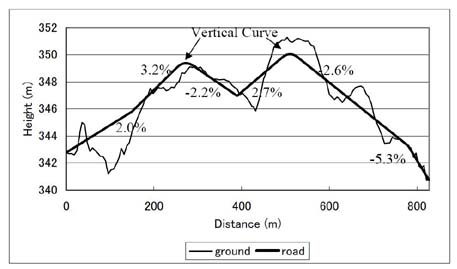
Figure 1. Forest road profile of fixed horizontal alignments with five grade change points.
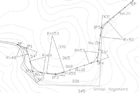
Figure 2. Forest road plane showing contour intervals, horizontal alignment, and 30-m road stations (= and indicate an existing road and an extended road, respectively).
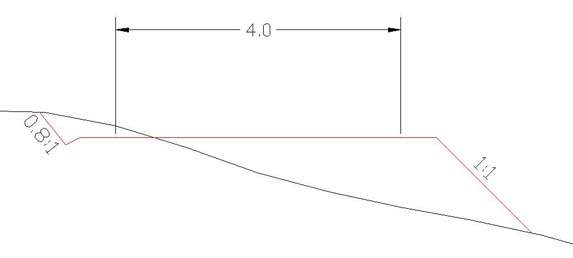
Figure 3. Cross section.
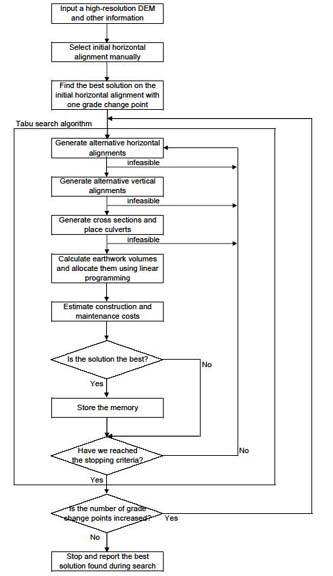
Figure 4. Flowchart of the model.
Objective Function
The objective function that minimizes the total cost, TC takes the following form:
Min TC=C+M0 (1)
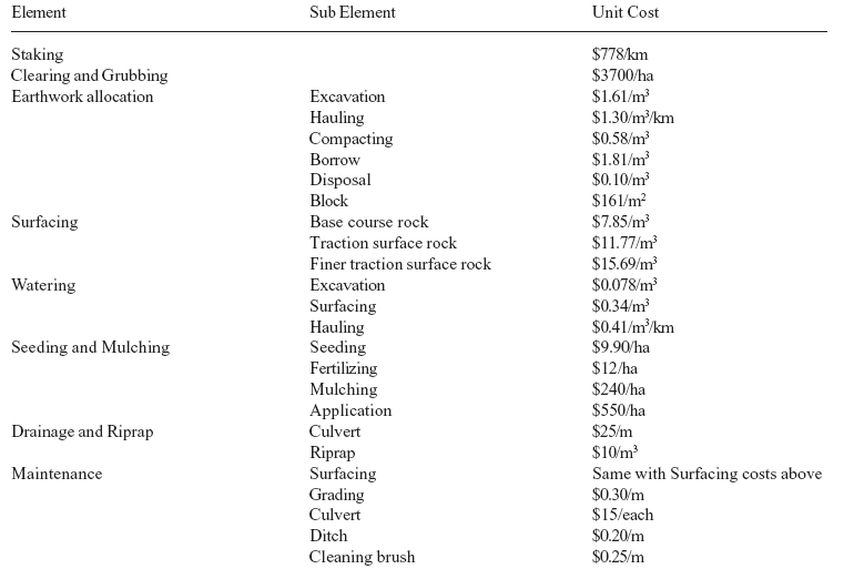
where C is the construction cost and M0 is the discounted maintenance cost. The total cost of each road section is determined using the method of Akay [2], considering construction and maintenance activities. The road construction cost is computed for the following activities: construction staking, clearing/grubbing, earthwork allocation, drainage and riprap, surfacing, water supply/watering, and seeding/mulching. The maintenance activities consist of rock replacement, grading, culvert/ditch maintenance, and brush clearing. The discounted cost of future road maintenance is estimated to compare the total construction and discounted maintenance cost for alternative alignments. The USDA Forest Service Region 6 Cost Estimating Guide [29] is used to estimate the costs (Table 1).
Table 1. Unit costs.

Display large image of Table 1
Earthwork Allocation
Cross sections are required to compute an earthwork volume (Figure 3). In this study, the following dimensions are used to design cross sections: 4.0m road width, 0.8:1 cut slope, and 1:1 fill slope. Ground elevations on both sides of each cross section are estimated at an interval of 1m horizontal distance from the road center using bilinear interpolation. In addition to those elevation points along a cross section, ground elevations are estimated at the edges of roads, ditches, cut slopes, and fill slopes. The area of a cross section is calculated from the geometry of natural ground and the road template. In order to accurately calculate earthwork volume for curved roadways, an eccentricity of a cross section along a curve is also calculated [13]. The eccentricities are calculated by taking the moments about the roadway centerline.
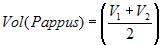
Earthwork volume of straight roadways can be computed using the average end-area method. With this method, the volume is computed by multiplying the distance between cross sections by the average of the end cross-sectional area. The Pappus-based method is used to compute earthwork volume for a road section on a horizontal curve [13]. This method estimates the volume as the average volume resulting from rotating the areas of the two cross sections about an axis in their planes.
 (2)
(2)
 (3)
(3)
 (4)
(4)
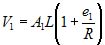
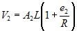
Vol is the earthwork volume (m3) between cross sections 1 and 2, L is the distance (m) between the cross sections, and R is the horizontal curve radius (m). V1 and V2 are volumes (m3) of rotation of cross sections 1 and 2, respectively, A1 and A2 are the areas (m2) of cross sections 1 and 2, respectively, and e1 and e2 are eccentricities (m) of cross sections 1 and 2, respectively. The sign of the eccentricity is positive if it is outward from the curve centerline and negative if it is inward.
Aruga et al. [5] found that the Pappus-based method provides more accurate earthwork volume than the end-area method and that the results of the method were similar to the earthwork volumes estimated by Monte Carlo simulation [13] when the horizontal distance between cross sections was less than 6 m. The economic distribution of cut and fill quantities is determined using the linear programming method of Mayer and Stark [19].
Geometric Constraints
The maximum gradient of roads is limited to 18% in this study considering truck performance. The gradient must also be greater than 2% to provide adequate water drainage. If the absolute value of the grade change between two consecutive road segments is more than 5%, a vertical curve is placed to smooth out the abrupt grade change (Figure 1). A minimum curve length of 20 m is used. To determine a feasible curve length, crest and sag vertical curves are considered separately depending on whether the curve length is greater or less than the Stopping Sight Distance (SSD) [20].
 (5)
(5)
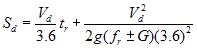
Here, Sd is the SSD (m), Vd is the design speed (e.g. 30 km/h), tr is the perception-reaction time (2.5 seconds), g is the gravity (9.81 m/sec2), fr is the braking tractive coefficient (e.g. 0.5), and G is the road grade (decimal). On one-lane, two-directional roads, the SSD is approximately twice the SSD for a two-lane road because both drivers must safely stop their vehicles. The length of the crest vertical curve is calculated based on the SSD. When the SSD is greater than curve length,
 (6)
(6)
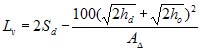
when the SSD is less than the curve length,
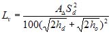 (7)
(7)
where Lv is the length of vertical curve (m), A) is the algebraic difference in grades (percent), hd is the height of driver's eye above road way surface (1.05 m), and ho is the height of object above roadway surface (0.15 m). The length of a sag curve is calculated based on the SSD as well. When the SSD is greater than the curve length,
 (8)
(8)
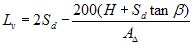
and, when the SSD is less than the curve length,
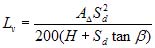 (9)
(9)
where H is the head light height (0.6 m) and $ is the upward angle of the headlight beam (1 degree).
A simple circular horizontal curve is designed to provide a transition between two straight roadway sections (Figure 2). The minimum curve radius of 18 m is generally used for a truck with trailer on forest roads. The SSD is computed using the limiting speed of the vehicle around the horizontal curve.
Vlimit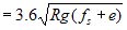 (10)
(10)
Here, Vlimit is the limiting speed (km/h), R is the curve radius (m), fs is the coefficient of side friction (e.g. 0.1), and e is the superelevation of the horizontal curve. It is assumed that a horizontal curve is not feasible in the model if the distance between two adjacent curves is less than 10 m and the curve length is less than the SSD. Thus, the first assumption restricts a maximum radius and the second restricts a minimum radius. It is also assumed that the road grade remains constant along horizontal curves.
A minimum lateral clearance distance from the center of the vehicle lane is required for a vehicle operator to see the length of curve equal to the required safe SSD around the curve. A 0.6 m height of object at the mid-ordinate point is used if a cut slope obstructs the line of sight.
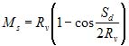 (11)
(11)
Here, Ms is the mid-ordinate (m) and Rv is the design curve radius minus the half of the road width (m). This condition assumes that there is little or no vertical curvature on the horizontal curve. If cut slope height is higher than the height of object, the model lays back the cut slope from road edge to the driver's line of sight to provide the minimum SSD [20]. In order to layback the cut slope, the horizontal distance from each point to the line of sight, Mp (m) is computed.
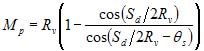 (12)
(12)
where
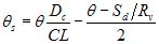 (13)
(13)
where 2 is the intersection angle (radian), Dc is the horizontal distance from the beginning point of the curve to each point of the curve (m), and CL is the curve length (m).
Curve widening should be considered to provide adequate lane width for the off-tracking of critical design vehicles, such as log trucks, tractor trailer trains, and logging equipment. The off-tracking equation proposed by Cain and Langdon [8] was used to compute off-tracking of a truck tractor with semi-trailer and a truck tractor with stinger-steered trailer (pole trailer).
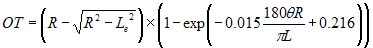 (14)
(14)
Here, OT is the total vehicle off-tracking (m) and Le is the effective vehicle length (m). The effective vehicle length for a tractor semi-trailer combination is:
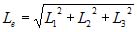 (15)
(15)
where L1 is the wheelbase of the tractor (e.g. 4.72 m), and L2 is the distance from the fifth wheel to the center of the rear duals of the first trailer (e.g. 11.67 m). The offset to the kingpin is assumed to be zero. If a second trailer is being pulled, then L3 is the distance from the fifth wheel to the center of the rear duals of the second trailer. For a stinger-steered trailer, L2 is the length of the stinger and L3 is the bunk-to-bunk distance minus the length of the stinger. For the stinger-steered trailer, L22 is subtracted rather than added. We assume the design vehicle is the truck tractor with semi-trailer.
The USFS Preconstruction Handbook [28] recommends a straight line taper transition that begins before the curve and ends after the curve. Turnouts are designed to facilitate vehicle passage at an interval of 300 meters [1]. The turnout should be at least 3 meters in width and 15 meters long with a 7.5-meter transition at each end.
OPTIMIZATION PROCEDURE
Tabu Search Algorithm
Tabu Search is a solution strategy for combinatorial optimization problems [14] and has evolved from gradient search algorithms [15]. Gradient search algorithms can guarantee an optimal solution when the solution space is convex. However, many real-world combinatorial problems do not have a convex solution space, and others are also discrete. Tabu Search can systematically look for feasible solutions to both discrete and non-convex problems. The key capability of Tabu Search is that it remembers the choices it makes, which is not a common in traditional gradient search algorithms. This memory is used to force the exploration of other areas of the solution space, thus increasing the chance of locating a good solution. Tabu Search procedures can involve several phases. Common to all Tabu Search procedures is an initial phase known as the "short term memory phase" and is followed by subsequent phases which use information accumulated during the initial search phase to guide either future intensification or diversification of the search or both. Our Tabu Search procedure involves a short term memory phase followed by an intensification strategy. We start with a discussion of the short term memory phase, followed by an intensification phase, and discuss opportunities to diversify the search later.
We first select intersection points for an initial horizontal alignment manually (Figure 4). With one grade change point, the model searched for all alternatives by changing the placement and heights of grade change points while the horizontal alignment is fixed. Then, the best solution is used to initiate the Tabu Search algorithm to optimize horizontal and vertical alignments simultaneously with one grade change point. After the Tabu Search algorithm finds the best solution with one grade change point, it continues to search from the best solution as the initial solution with two grade change points. In other words, different numbers of grade change points were considered using the following steps in the optimization process: 1) Tabu Search began with a small number of grade change points and finds the best road alignment, 2) the number of grade change points is increased by one, 3) Tabu Search was again applied to find the best solution with the increased number of grade change points. The best solution found at the previous step (Step 1) was used as the initial solution at Step 3.
For each iteration of Tabu Search, a neighborhood, which is a set of new feasible solutions, is created by slightly changing the previous feasible solution (Figure 5). Tabu Search operates by selecting "candidate" decision choices from a "neighborhood". If the candidate decision choice is tabu (i.e. it has been selected previ ously), then it is rejected and the next top candidate is selected. Rules, called aspiration criteria, can be set to allow consideration of candidate choices that are tabu. Aspiration criteria allow further consideration of tabu candidate choices if the inclusion of the choice in the current solution will result in a solution that has an objective function value, which is better than any of the previously observed objective function values.
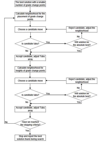
Figure 5. Flowchart of Tabu Search algorithm for vertical alignments.
If the choice is not tabu, the candidate choice is formally brought into the solution, and the resulting solution's objective function value is compared against the best previously observed objective function value (stored in memory). If the resulting solution is better than the previous best solution, it is saved as the best solution.
The algorithm moves forward one iteration with the inclusion of the candidate choice in the solution. If the resulting solution is not better than the previous best solution, the algorithm moves with the candidate which will produce the maximum positive gain in the objective function value. If a positive gain is not possible, the algorithm moves with the candidate which will produce the least decline in the objective function value. Thus, the search is not constrained at the local optima.
The tabu list is developed to keep track of choices which have been recently made. In the first iteration, the tabu values in the tabu list are all zero. The formally accepted solution is given an initial tabu value. After each iteration of the model, the tabu value is decreased by one. When the tabu value equals zero, the solution restricted by tabu is not considered tabu, and will not be subject to the tabu restriction. In Tabu Search, this is called short-term memory. Short term memory essentially diversifies the search by keeping the model from cycling back to a local optimum that has already been identified. Some Tabu Search applications use a dynamic tabu tenure value although we do not use it in this study.
Neighborhood Definition
In our case, the model generates neighborhood solutions by changing the locations of intersection points, radii of horizontal curves, and the placement and heights of grade change points. The locations of intersection points are separated into North-South and East-West coordinates and examined. Neighborhood solutions of North-South coordinates of intersection points are generated at an interval of 1-meter within 5-meter zones around the previous North-South coordinates of intersection points. Neighborhood solutions of East-West coordinates of intersection points are generated as well. Neighborhood solutions of radii of horizontal curves are generated at an interval of 1-meter within 5-meter zones around previous horizontal curve radii. Note that neighborhood solutions of radii are limited between minimum and maximum radii. The model examines the placement of grade change points by selecting candidates from stations on straight roadways. It does not select candidates from stations on curved roadways because it is assumed that the road grade remains constant along horizontal curves. It also generates neighborhood solutions by changing the heights of grade change points at an interval of 1-meter within 5-meter zones around elevations of grade change points.
We illustrate the neighborhood definition using an example for heights of five grade change points. In the first iteration,
height(-1,2,5,-4,4)
Tabu list=(0,0,0,0,0)
A neighborhood is:
(-5,2,5,-4,4), (-4,2,5,-4,4),—(5,2,5,-4,4)
(-1,-5,5,-4,4), (-1,-4,5,-4,4),—(-1,5,5,-4,4)
(-1,2,-5,-4,4), (-1,2,-4,-4,4),—(-1,2,4,-4,4)
(-1,2,5,-5,4), (-1,2,5,-3,4),—(-1,2,5,5,4)
(-1,2,5,-4,-5), (-1,2,5,-4,-4),—(-1,2,5,-4,5)
If the change of the second grade change point from 2 to 4 is feasible with respect to the constraints and represents the best possible improvement in the objective function value or the least deterioration of the objective function value, it is given a tabu tenure value (e.g. 3).
height(-1,4,5,-4,4)
Tabu list=(0,3,0,0,0)
After each iteration of the model, the tabu tenure value is decreased by one.
Based on computation experience we terminate the initial short term memory phase after 1000 iterations. An intensification strategy is then implemented which is accompanied by a redefinition of the neighborhood. The neighborhood for the intensification stage is generated by changing vertical heights of grade change points at an interval of 0.1m within ±1 m around the selected alignment. The placement of intersection points and grade change points is fixed during the second search process. This second search process stops after a specified number of iterations (e.g. 100). This second search process refines the best solution found from the first process and provides a better solution for the final best alignment. Some Tabu Search applications use a memory-based method for signaling when to intensify the search and when to terminate the search. Through computational experience on this problem, we have chosen to explicitly define the intensification and termination points.
APPLICATION
Study Site
The road design model developed in this study was applied to a part of Capitol Forest in western Washington State. Most of the study area is covered by 70-year-old coniferous forests. The elevation range is from 150 m to 400 m with the ground slopes of 0% to 100%. This area was mapped by a small footprint LiDAR system (Table 2) in the spring of 1999 and the LiDAR data was converted into a 1.52 m x 1.52 m grid DEM. The orthophotographs of the study area were generated based on airphotos, which were taken four months before the LiDAR data (Figure 6).
Table 2. Flight parameters and scanning system setting.
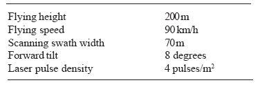
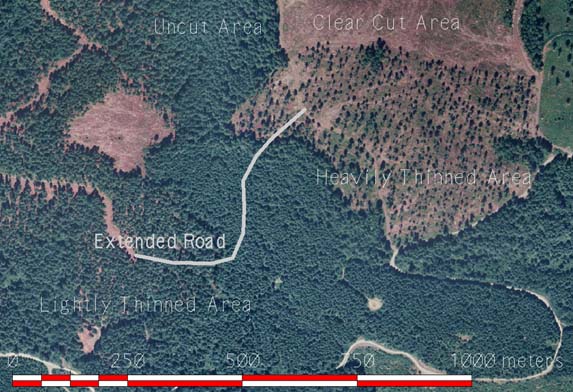
Figure 6. Study site (orthophotograph courtesy of the Washington State Department of Natural Resources, Resource Mapping Section).
When Reutebuch et al. [25] assessed the vertical accuracy of the LiDAR system using 348 sample points surveyed by a Total Station, the resulting root-mean-square error was 0.43 m. When Aruga et al. [3] evaluated the vertical accuracy of the LiDAR on the forest road in the same site, the result showed that the root-mean-square error was 0.14 m (Figure 7). The difference between the results from Reutebuch et al. [25] and Aruga et al. [3] might be caused by forest cover which may prevent light pulses from reaching the ground. The root-mean-square error of 0.14 m on forest road might be the error of the LiDAR system itself [23].
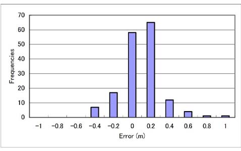
Figure 7. Difference between Total Station survey and LiDAR measurement.
Optimization of Horizontal and Vertical Alignments
After the study site was measured by LiDAR and the orthophotographs were generated in 1999, new road construction was planned to extend the existing forest road in the study site (Figure 6). The intersection points were manually identified and the forest road design model was applied to generate an initial horizontal alignment, subject to the given geometrical design constraints (Figure 2). As a result, the total length of the extended part of the road was 827 m, which was divided into 27 sections of 30-meter each.
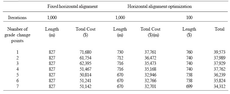
We have examined the effects of relocating grade change points with the fixed horizontal alignment [5]. Tabu Search found the best vertical alignment, which includes five grade change points (Table 3). Its total cost was $50,814. Then, the model simultaneously optimized horizontal and vertical alignments. The simultaneous optimization algorithm was able to find a better solution with seven grade change points. The total construction and maintenance cost was $32,701 (Table 3). Compared with the best solution of the fixed horizontal alignments, the total cost and the total road length were reduced by 36% and 19%, respectively.
Table 3. Costs with different numbers of grade change points.

Display large image of Table 3
The best solution of fixed horizontal alignments with five grade change points was $61.42/m. One quarter of the construction cost was earthwork cost and another quarter was surfacing cost (Table 4). On the other hand, the best solution of optimized horizontal alignments with seven grade change points was $48.74/m. Simultaneous optimization successfully reduced the total costs by $12.68/m of which $9.50/m was due to reduction of earthwork allocation cost. The forest road profile with fixed horizontal alignments has some differences between ground heights and road profile (Figure 2). The biggest difference occurred at the 100-m point from the start point. The difference was about 4 m. The forest road profile with optimized horizontal alignments followed the ground profile (Figure 8). The program found a smoother ground profile as changing the location of intersection points. Thus, the program generated a better vertical alignment.
Table 4. Best costs ($/m).
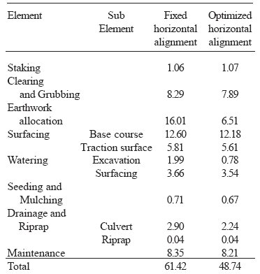
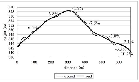
Figure 8. Forest road profile of optimized horizontal alignment with seven grade change points.
Moreover, the amount of material moved from borrow area was reduced from 2,573.25 m3 of fixed horizontal alignments to a negligle amount (1.75 m3 ) with the optimized horizontal and vertical alignments. As a result, the model could balance fill and cut volumes in this section.
DISCUSSION
Stopping Criteria
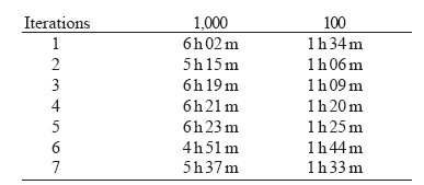
The search process to optimize horizontal and vertical alignments indicated that Tabu Search obtained a large improvement within a few iterations because Tabu Search uses a modified gradient search technique (Figure 9). However, sometimes it continued to find improvements after several hundred iterations. For example, Tabu Search with one grade change point found better solutions at the 400th and 600th iterations. The gains at the 400th and 600th iterations were $1,127 and $558, respectively. A total gain during search process was $53,675, calculated from an initial solution with one grade change point, $86,376 and an optimum solution with seven grade change points, $32,701. Therefore, gains at the 400th and 600th iterations were 2.1% and 1.0% of a total gain during search process, respectively. Similarly, the gain with five grade change points at the 400th iteration was 2.6%. The program was conducted with a Pentium 4 2.4 GHz desktop computer. The search process for each number of grade change points took four to eight hours depending on the number of grade change points and the number of feasible solutions generated during search process (Table 5). These imply that Tabu Search optimization dramatically improves the solution quality at an earlier stage, but once it finds a good solution it takes a large amount of time to further improve the solution quality. Therefore, we should consider the trade-off between computational time and solution quality.
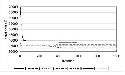
Figure 9. Search process with different numbers of grade change points.
Since Tabu Search obtained a large improvement within 100 iterations, we examined the effect of reducing the number of the first search process iterations to 100 instead of 1,000, on the results. Tabu Search found slightly worse solutions during 100 iterations than those during 1,000 iterations (Table 3). The difference between the results during 100 iterations and 1,000 iterations with seven grade change points was 5%. However, the result during 100 iterations was 32% better than the best solution with fixed horizontal alignment. Although computing times for 100 iterations did not proportionally reduce the time to one tenth of the time for 1,000 iterations, computing time was significantly reduced (Table 5). Therefore, it might be a better option to use the number of iterations as 100 for less computing time even though Tabu Search found slightly less quality of solutions.
Table 5. Computing time with different numbers of grade change points
Tabu Search Procedure
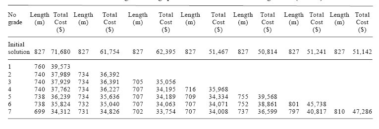
We examined effects of initial solutions for Tabu Search algorithm on solution quality and computing time. We ran the Tabu Search heuristic with 100 iterations, starting with the best solution with a specified number of grade change points on the fixed horizontal alignment (Table 3). The result showed that Tabu Search from better initial solutions found relatively better final solutions (Table 6). Tabu Search algorithm starting from the best solution with one grade change point on the fixed horizontal alignment, $71,680 (Table 3) found the best solution with seven grade change points on the optimized horizontal alignment, $34,312 (Table 6). On the other hand, Tabu Search algorithm starting from the best solution with three grade change points on the fixed horizontal alignment, $62,395 found the best solution with seven grade change points on the optimized horizontal alignment, $33,754. However, to use this method, Tabu Search optimization must be conducted to search for the best solution with each number of grade change points on fixed horizontal alignments. Then, Tabu Search optimization must be conducted again using the best solution with each number of grade change points on fixed horizontal alignments as the initial solution in order to find the final solution. Although this method finds a good solution, it can be considered to be time consuming. Therefore, we could not recommend this method to find a good solution.
Table 6. Total costs with 100 iterations of Tabu Search optimization starting from the different initial solutions found with the different number of grade change points on the fixed horizontal alignments (Table 3).

Display large image of Table 6
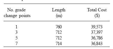
As an alternative to sequentially solving for additional grade change points, we examined another method to shorten the Tabu Search optimization time. We had conducted the Tabu Search by: 1) finding the best road alignment, 2) increasing the number of grade change points by one, 3) and using the best solution found at the previous step (Step 1) as the initial solution in order to find the best solution with the increased number of grade change points. As an alternative, we increased the number of grade change points by two or more at Step 2. For example, we used the set of grade change points (1, 3, 5, 7) instead of considering all grade change points (1, 2, 3, 4, 5, 6, 7) in order to shorten computing time (Table 7). Although this method did not provide a better solution than Tabu Search optimization looking at all grade change points (Table 3), this method clearly shortened computing time. This is very important for problems larger than the example of seven grade change points used in this study. This method should be examined again for larger problems based on computing time and solution quality.
Our procedure has used a Tabu Search with short term memory followed by an intensification procedure. Diversification currently relies on the user to specify the number and location of intersection points for the horizontal alignment and the number of grade change points for the vertical alignment. To assist the user, the number and location of intersection points for the horizontal alignment and the number of grade change points for the vertical alignment could form additional decision variables. Future work could examine a hybrid approach. For example, to avoid manually initializing intersection and grade change points, we could use random search, to assign the numbers and locations of intersection and grade change points, and the Tabu Search procedures presented here, to minimize the total construction costs.
Table 7. Total costs when only 1, 3, 5, and 7 grade change points were considered.
CONCLUSIONS
We have developed a forest road design model that simultaneously optimizes horizontal and vertical alignments of forest roads. Once intersection points for an initial horizontal alignment are established, the model generates alternative horizontal and vertical alignments for each forest road section and locates the cross sections along the road prism. The model also estimates earthwork volume and computes construction and maintenance costs for given road alignments and their spatial locations. The model then optimizes road alignments based on construction and maintenance costs using a Tabu Search algorithm. The model could generate the ground profile and cross sections precisely due to a high resolution DEM from LiDAR. The model could accurately calculate earthwork volumes for curved roadways with the Pappus-based method.
The model was applied to a part of Capital State Forest in Washington State. Although the verification of the solutions was limited, the case study indicated that the program could generate feasible and good road alignments. The accuracy of generating ground profile and calculation of earthwork volume depends on a high resolution DEM. Low resolution DEM will result in lower accuracy of the generated ground profile and calculation of earthwork volume and may not yield useful estimates. Rock excavation can be an important cost. Using LiDAR alone, we do not know the presence of rock from a high resolution DEM. Incorporation of soil and rock information as well as other attributes such as other geographic attributes such as stream, wildlife habitat, and slope stability, etc, could make the model a practical tool for a forest road design. Future work should include developing a method to estimate transportation costs. Transportation cost, even on low volume forest roads, can be an important factor of road design and could be considered when road alignment is optimized.
ACKNOWLEDGEMENTS
LiDAR data were provided by the USDA Forest Service, PNW Research Station, Resource Management and Productivity Program. The orthophotograph shown in Figure 6 is courtesy of the Washington State Department of Natural Resources, Resource Mapping Section. We would like to express our appreciations to Mr. Steve Reutebuch, Mr. Robert McGaughey, and Dr. Ward Carson with USDA Forest Service and Professor Edwin S. Miyata with University of Washington for their willingness to provide the LiDAR data and to help with data process, and WADNR for letting us use the study site in Capitol Forest.
AUTHOR CONTACT
Professor Aruga can be reached by e-mail at --
aruga@cc.utsunomiya-u.ac.jp
REFERENCES
[1] AASHTO. 1994. A policy on geometric design of highways and streets, Washington, DC.
[2] Akay, A.E. 2003. Minimizing total cost of construction, maintenance, and transportation costs with computer-aided forest road design. PhD thesis, Oregon State University, Corvallis.
[3] Aruga, K. and E.S. Miyata. 2004. Application of airborne laser scanner to forest road survey. J. Jpn. For. Eng. Soc. 19(1): 49-54. (in Japanese).
[4] Aruga, K., J. Sessions, and A.E. Akay. 2005. Heuristic techniques applied to forest road profile. J. For. Res. 10(2): 83-92.
[5] Aruga, K., J. Sessions, and A.E. Akay. Application of an airborne laser scanner to forest road design with accurate earthwork volumes. J. For. Res. 10(2): 113-123.
[6] Bettinger, P., J. Sessions, and K. Boston. 1997. Using Tabu Search to schedule timber harvests subject to spatial wildlife goals for big game. Ecol. Model. 94: 111-123.
[7] Bettinger, P., J. Sessions, K.N. Johnson. 1998. Ensuring the compatibility of aquatic habitat and commodity production goals in eastern Oregon with a Tabu Search procedure. For. Sci. 44(1): 96-112.
[8] Cain, C. and J.A. Langdon. 1982. A guide for determining minimum road width on curves for single-lane forest roads. Engineering Field Notes, Volume 14, USDA Forest Service.
[9] Chew, E.P., C.J. Goh, and T.F. Fwa 1989. Simultaneous optimization of horizontal and vertical alignments for highways. Transp. Res. B. 23(5): 315-329.
[10] Chung, W., J. Sessions, and H.R. Heinimann. 2004. An application of a heuristic network algorithm to cable logging layout design. Int.. J. For. Eng. 15(1): 11-24.
[11] Coulter, E.D., W. Chung, A. Akay, and J. Sessions. 2002. Forest road earthwork calculations for linear road segments using a high resolution digital terrain model generated from LIDAR data. Proc. First Precision Forestry Symposium: 125-129.
[12] Dowsland, K.A. 1993. Simulated Annealing. In: Reeves, C. [Eds] Modern heuristic techniques for combinatorial problems. Blackwell Scientific Publications, Oxford. pp 20-69.
[13] Easa, S.M. 2003. Estimating earthwork volumes of curved roadways: simulation model. J. Surveying Eng. 129(1): 19-27.
[14] Glover, F. 1989. Tabu Search-Part I. ORSA J. Computing 1: 190-206.
[15] Glover, F. and M. Laguna. 1993. Tabu Search. In: Reeves, C. [Eds] Modern heuristic techniques for combinatorial problems. Blackwell Scienrific Publications, Oxford, pp.70-150.
[16] Goh, C.J., E.P. Chew, and T.F. Fwa. 1988. Discrete and continuous model for computation of optimal vertical highway alignment. Transp. Res. B. 22(9): 399-409.
[17] Howard, B.E., Z. Bramnick, and J.F.B. Shaw. 1968. Optimum curvature principle in highway routing. J. Highw. Div., Am. Soc. Civ. Eng. 94(1): 61-82.
[18] Kanzaki, K. 1973. On the decision of profile line of forest road by dynamic programming. J. Jpn. For. Soc. 55: 144-148. (in Japanese).
[19] Mayer, R. and R. Stark. 1981. Earthmoving Logistics. J. Const. Div. 107(CO2): 297-312.
[20] Mannering, F.L. 1990. Principles of highway engineering and traffic analysis. John Wiley & Sons, Inc. New York.
[21] Murphy, G. 1998. Allocation of stands and cutting patterns to logging crews using a Tabu Search. J. For. Eng. 9(1): 31-37.
[22] Nicholson, A.J. 1976. A variational approach to optimal route location. J. Highway Eng.: 22-25.
[23] Omasa, K., Y. Akiyama, Y. Ishigami, and K. Yoshimi. 2000. 3-D remote sensing of woody canopy heights using a scanning helicopter-borne LiDAR system with high spatial resolution. J. Remote Sensing Society of Japan 20(4):34-46. (in Japanese with English summary).
[24] Reeves, C. 1993. Genetic Algorithms. In: Reeves, C. [Eds] Modern heuristic techniques for combinatorial problems. Blackwell Scientific Publications, Oxford, 151-196.
[25] Reutebuch, S., R.J. McGaughey, H-E. Andersen, and W. Carson. 2003. Accuracy of a high-resolution LiDAR-based terrain model under a conifer forest canopy. Can. J. of Remote Sensing 29(5):1-9.
[26] Richards, E.W. and E.A. Gunn. 2000. A model and Tabu Search method to optimize stand harvest and road construction schedules. For. Sci. 46(2): 188-203.
[27] Trietsch, D. 1987. A family of methods for preliminary highway alignment. Transportation Science 21: 17-25.
[28] USDA Forest Service. 1987. Road preconstruction handbook. Forest service handbook No. 7700.56.
[29] USDA Forest Service. 1999. Cost Estimating Guide for Road Construction Region 6. Oregon, Portland.