Vol. 16 No. 2 July 2005
M. Forsberg
M. Frisk
The Forestry Research Institute of Sweden
Uppsala, Sweden
M. Rönnqvisty
The Forestry Research Institute of Sweden
Uppsala, Sweden
and
Linköping Institute of Technology
Linköping, Sweden
The authors are, respectively, Researchers at the Forestry Research Institute of Sweden (Skogforsk). Rönnqvist is also a Professor at the Linköping Institute of Technology.
ABSTRACT
We report on the development of a new decision support system for transportation planning in Swedish forestry. The system deals both with strategic and tactical decisions. Strategic decisions concern usage of train system, terminal location and capacity, and wood bartering between companies and/or organizations. In tactical planning we consider decisions on catchment areas, destination of supply points and potential back-haulage routes. The system uses a GIS-based map user-interface. Two important modules in the system are the new Swedish road database and an optimization module consisting of a suite of models and methods. The development has included several organizations and forest companies. We discuss two case studies at participating companies that illustrate the usage of the system.
Keywords: Transportation, optimization, forestry, linear programming, decision support system.
INTRODUCTION
We consider the planning of transportation activities occurring in forestry from supply points in harvest areas to demand points at industries, such as pulp-, paper- and sawmills. Transportation is carried out by logging trucks or trucks combined with railway transportation for longer distances. It is an important part of the overall forest wood chain (or supply chain). In Sweden it represents approximately 25% of all domestic transport by truck and railway.
The cost of transportation represents one third of the total cost of raw material, round wood, to the forest industry.
The management of these activities is commonly divided into three perspectives: strategic, tactical and operational. The strategic management deals with adjusting the capacity or organization of transportation with respect to changes in production and demand. Examples are introduction of train systems, new terminals and co-operation with other companies. The time horizon is often several years. Tactical management deals with changes of a shorter time horizon, a few months to a year. Examples are capacity changes in train system, new catchment areas and establishing potential back haulage routes. Operational management deals with problems of a few hours to a few weeks time horizon. Planning the work schedule for next week's deliveries of an individual truck driver is one example. There are many articles written about different OR problems arising with these activities. Several of these are discussed in Martell et al. (1998) and Rönnqvist (2003).
In Figure 1 we illustrate the general problem. In this example we have two industries and a number of supply points that deliver logs to the industries. Transportation is either carried out directly with trucks or in a combination of trucks and trains where trucks are used for the transportation to/from terminals. There are a number of strategic and tactical questions to be answered in order to find the best possible transportation plan. Typical strategic and tactical questions are listed below.
Current transportation planning in Sweden is often manual and decentralized to districts. Catchment areas are decided by matching supply points with demand points i.e. destination of logs. Train planning is done separately where overall volumes through terminals and train system are decided. These volumes are then used as new additional demand and supply points for the truck planning. There is however a large potential for improved efficiency. Several studies, where OR models are used, have shown potential cost reductions of 5 to 10 percent with a better management of the transportation, see e.g. Carlsson and Rönnqvist (1998), Forsberg (2003) and Eriksson and Rönnqvist (2003). Savings come from a combination of improvements. Typical examples are; better catchment areas i.e. better match between supply and demand points, better use of back-haulage tours, better co-ordination between districts and/or companies.

Figure 1. Illustration of the general transportation problem. The transportation is carried out through the use of a combination of trucks and trains.
It is very time consuming to perform these studies. They require the use of several steps of processing with different software packages. A lot of manual work to set up and maintain data is also required. It is therefore difficult to use in practice by transportation and logistics managers. In a joint research and development project running through 2002-2004 the FlowOpt system was developed. One aim was enable integrated planning between trucks and train systems, as well as co-ordination between several companies. Other aims were to use new information systems and limit the time needed to solve, analyze and generate result reports e.g. maps for a case study. A final aim was to develop a system that by itself or parts of it could be used directly in the planning process by managers in forest companies. The system development is a co-operation between The Forestry Research Institute of Sweden, Linköping University, the Swedish Agency for Innovation System, software companies Optimal Solutions and Dianthus and five large participating forest companies; Stora Enso, SCA, Södra Skogsägarna Holmen Skog and Sveaskog. In this paper we describe the resulting system and experiences from two case studies.
The outline of this paper is as follows. First, in Section Problem Description, we describe the basic problem and important and practical features needed for a complete model description. This include train systems, back-haulage routes and co-operation between companies. In Section Model and Solution Methods we develop the overall model. In Section System Description we describe the system and some of the important components including the road database and optimization modules. In Section Case Study we discuss two case studies. One is focused on strategic issues for integrated planning between trucks and train. The second relates to wood bartering between two companies. Finally we make some concluding remarks.
PROBLEM DESCRIPTION
Transportation Planning Using Transportation Models
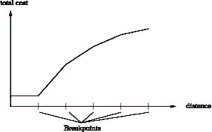
An important quantitative tool in transportation planning is the "classical" transportation problem with variables representing the flow from supply point i to demand point j", constraints on supply and demand and where the objective is to minimize total costs. In forestry there are several assortments (depending on e.g. species and dimensions). For the circumstance that industry demands can be more or less specific regarding assortments, so-called assortment groups can be used to specify the demands. A demand for an assortment group can then be fulfilled by one or several different assortments, depending on the definition of the assortment group. Supply points can be individual harvest units or an area of several harvest units. The latter is more common for strategic planning over a large area or for an entire company. Demand points are industrial need at a mill such as pulp-, paper- and saw-mills. The transportation cost is based on negotiations between forest companies and hauliers. The cost is typically based on a cost function with a number of break points at specified distances. An illustration is given in Figure 2.
Figure 2. Illustration of a typical transportation cost function.
The above problem can be formulated in a Linear Programming (LP) problem. For a typical planning problem we may have 500-700 supply points, 100-200 demand points, 5-10 assortments and 5-15 assortment groups. Only a few of the potential number of variables and constraints are used. Potentially we have 21 million (700*200*10*15) variables and 10,000 (700*10+200*15) constraints for such a case. However, in practice, each assortment group typically involve 1-3 assortments and each industry typically only have 1-3 demands. For a typical problem when we have filtered out the possible variables and constraints we end up with 50- 100,000 variables and 3-6000 constraints. The problem is typically efficiently solved by any commercial LP-solver. The main problem is instead to collect correct and relevant information. Demand at industry is normally straightforward to collect but supply information of assortments are more difficult to gather. This is because there are different ways to inform about harvest operations. Some are more detailed and some are just estimates (and in some cases very crude). Correct information about transportation distances is also difficult to collect. In the FlowOpt system we use a new national road database to collect distance information. It consists of all roads (private as well as governmental) in Sweden.
A typical application of such model is to decide catchment areas for industries. In Figure 3 (left) we illustrate this with a case where we have five pulp mills and a set of harvest areas. Each mill has a demand of a particular pulp log (one assortment). Each area has a specific supply and each industry a given demand. If we solve the model we may get the solution in Figure 3 (right) where we have indicated the catchment areas for each industry. In this case we can note that distances between supply and demand is critical and that each industry comes in the "middle" of each of the five areas.
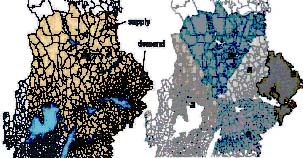
Figure 3. Illustration of catchment areas for one assortment. In the left part all supply areas are given together with industrial demand. In the right part each industry's catchment area is given.
Back-Haulage Tours
In a transportation model, the cost is based on the fact that the truck drives full from supply to demand point and empty in the other direction. This gives an efficiency of just 50%. Efficiency would be improved if routes involving several loaded trips were used, i.e. back-hauling. Backhauling refers to when a truck that has carried one load between two points, carries another load on its return. Traditionally, a truck travels loaded from a supply point to a demand point and then returns empty back to the source. The possibilities for back-hauling are somewhat limited in forestry. It must exist wood flows going in opposite directions. These flows in opposite direction do however occur since paper and sawmills demand different assortments - therefore not all supply points are coupled to the closest mill. The geographical distribution of mills is important in this context. In Figure 4 we provide such an example. Here, the backhaulage trip (bottom) goes "Norra - Heby (sawmill)-Västerås-Hallstavik (pulp mill)". The alternative is to use two direct trips (top). One trip is to go back and forward between "Norra-Heby" and the other to go back and forward between "Västerås-Hallstavik". The backhaulage trip is clearly shorter than the combined length of the alternative to use two direct trips.
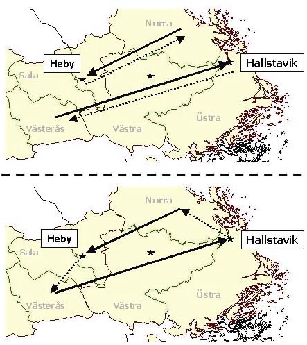
Figure 4. Illustration of a backhaulage route (bottom) based on two direct routes (top).
To use back-haulage tours can dramatically decrease the cost. Savings between 2-20% are reported in different analyses, see e.g. Carlsson and Rönnqvist (1998) and Forsberg (2003). The main problem with back-haulage routes is the huge increase in variables. If we have, say, 100,000 direct flows, then we get ten billions variables representing potential back-haulage routes made up of two direct flows. However, not all give a shorter unloaded distance. However, for typical applications where a back-haulage route is at least 20% shorter than corresponding two direct flows, we get 0.5-30 million variables. As we cannot include such numbers of variables explicitly in the model we use special solution methods based on column generation where they are used implicitly. This is further discussed in Section System Description.
Railway Transportation
Transportation is not always entirely carried out by truck. Many forest companies operate over large areas and distances between supply areas and industries are long. In these cases, substantial savings can be achieved using train transportation for longer distances since the unit transportation cost often is much smaller. However, the fixed cost for an entire system must be considered. Trains run between terminals located along the rail lines, so at least the first part of the transport still has to be carried out by truck. Many mills are located along the railway, which allows them to get train deliveries without the need of truck the last part.
Typically, a train system has one or more possible terminals where timber can be loaded and often just one where it is unloaded. Figure 5 illustrate an example of how a set of train system can work. At each terminal, there is a fixed cost for opening and another for handling i.e. loading and unloading. There is also a cost depending on volume and distance travelled. The capacity of a system is decided by how many wagons in use and the frequency of the trips. There are also alternatives in how they operate. One alternative is that the train is loaded directly when it arrives to a terminal and then leaves as soon as possible. Another is that the wagons are placed at the terminals and get loaded during several days and then the locomotives arrive and take the wagons to unloading terminals. For each train system there is a fixed cost depending on the number of wagons and locomotives used. Different capacity levels give different fixed costs.
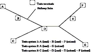
Figure 5. Illustration of a railway system with three train system.
Traditionally truck and train transportation have been planned separately. Typically, the train transportation is decided first. Then this plan in turn provide a new set of supply and demand points at the terminals when the trucks are planned in a second stage. The introduction of trains may give a very different structure of the catchment areas. Given the illustration given in Figure 3 we add two terminals and one train system that can load at the terminals and unload at one of the mills, see Figure 6. The impact after planning new catchment areas is that the areas get a very different geographical structure; this is illustrated in Figure 6.
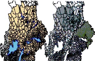
Figure 6. Illustration of catchment areas when two terminals and one train system is introduced.
Co-operation Between Companies
A strategic problem is to co-ordinate transportation planning for several companies that operate in the same region. It is very common that transport distances, and costs, can be decreased if companies exchange wood, apply bartering, between them. This issue is difficult as planners do not want to reveal supply, demand and cost information to competitors. In practice this is solved by deciding on wood bartering of specific volumes. Today this is done in an ad-hoc manner and is mostly dependent on personal relations. The model used in FlowOpt aims at handling such bartering in a flexible manner.
In Figure 7 we illustrate the potential benefits with wood bartering when two companies are involved. Here we have four mills at two companies (two mills each) together with a set of supply points for each company. In the left part each company operates by itself. The catchment areas are relatively large as compared to the right part where all supply and demand point are used on equal terms. In practice there are several restrictions imposed, for example, the bartering volumes are restricted, some mills are excluded, some supply points are excluded etc.
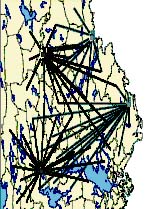
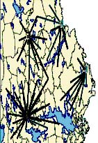
Figure 7. Illustration of wood bartering when the companies are illustrated with black and grey colours. In the left part each company operates by itself i.e. each company only use its own supply points for its demand. In the right part both companies uses all supply points as a common resource.
MODEL AND SOLUTION METHODS
Mathematical Model
In this section we describe the general model when train and truck transportation is integrated. It is based on the transportation problem described earlier but extended to take into account train and terminals. The index sets used in the LP-model are:
I : Set of supply points
J : Set of demand points
H : Set of assortments
G : Set of assortment groups
M : Terminals
Q : Train sets
Lq : Links in the railway system used by train set q
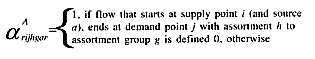
The direct truck flows are characterized by its starting point (supply point or terminal), its end point (demand point or terminal), the assortment, the assortment group the assortment is sorted to and the original source of the goods. Source can be either a specific company or a single supply point. We need the concept of source in order to be able to detect the catchment areas for each industries and when special restrictions are imposed on wood bartering. We introduce the set L as all possible start and end points, i.e. L= I ∪ J ∪ M. The direct flow variables using trucks are defined as
 = flow from location i and source
a to location j with assortment h to assortment group g
= flow from location i and source
a to location j with assortment h to assortment group g
The back-haulage flows are similar with the difference that there are two or more starting and ending points made up by several direct flows. We use the same definition of variables with the difference that we add index k to represent back-haulage route k. We note that each combination of back-haulage route k may have a set of combinations of I; j; h; g and a. If we for examplehave a back-haulage route consisting of two direct flows then for this k we have two sets of I; j; h; g and a. This indexing is used just to simplify and clarify the model.
 = flow in back-haulage route
k from location i and source
a to location j with assortment
h to assortment group g
= flow in back-haulage route
k from location i and source
a to location j with assortment
h to assortment group g
The train flows are defined in such a way that all combinations of flows on a train set is defined. For example, consider a train system, see Figure 8, where loading is done at terminals C and D, and unloading at terminals E and F. We then define physical flow variables for each of the combinations as is illustrated in Figure 8. In addition, we also include indices on assortment,assortment group, demand point and original source.
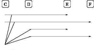
Figure 8. Example of how four physical flows are generated when there are two loading terminals and two unloading terminals.
 = flow with train set
q that load at terminal i, unload at terminal
j with assortment h to assortment group
g coming from original source a
= flow with train set
q that load at terminal i, unload at terminal
j with assortment h to assortment group
g coming from original source a
In order to get a robust model we include penalized variables that can handle any shortage appearing at the demand points, as given below. If these are not included in the model we might not find any solution and then no possibility to identify the problem. If any of these variables are non-zero in the solution it is easy to find out what the problem is, e.g. an error with the input data.
 = unfulfilled demand of assortment group
g at demand point j
= unfulfilled demand of assortment group
g at demand point j
Basic data about supply, demand and costs are needed. Since there may be different densities on assortments we have included a possibility to include this in the cost functions. Each backhaulage route has a cost based on the sum of the individual direct flows minus a bonus related to the savings in empty driving distance. The penalty cost for undelivered demand is just chosen high enough, for example, twice the largest transportation cost. All data is defined below.
sih : supply of assortment h at supply point i
djg : demand of assortment group g at demand point j
 : unit cost for truck transportation of assortment
h from node i to node j
: unit cost for truck transportation of assortment
h from node i to node j
 : unit cost for back-haulage route
k
: unit cost for back-haulage route
k
 : unit cost for train transportation on train set
q from terminal i to j
: unit cost for train transportation on train set
q from terminal i to j
 : penalty per undelivered unit of demand for
g at demand point j
: penalty per undelivered unit of demand for
g at demand point j
 : upper bound for total volumes on each railway
link (l) in train set q
: upper bound for total volumes on each railway
link (l) in train set q
 : inflow (unloading) capacity at terminal
m
: inflow (unloading) capacity at terminal
m
A very important aspect is what variables are included in the final model. Many variables are removed because they do not satisfy company rules or restrictions. Others are removed because they are unpractical. We can, for example, set up conditions like
In order to keep track of the filtering we can define coefficients
In order to keep the notation simple, we introduce a set RA which represents all variables xijhga defined. In the same way we introduce sets RB and RT for back-haulage routes and train flows, respectively. We also use the following simplified notation to represent a summation over index sets. The same is also used for sets RB and RT .
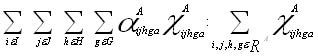
In order to keep track of physical flow of train system q that passes a certain link r in the railway system we use the set Rqr. This is simply the subset of variables in RT where we have fixed indices q and r.
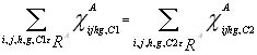
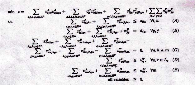
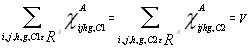
Constraint set (A) represent actual supply, set (B) demand, set (C) terminal balance, set (D) link capacity and set (E) terminal capacity. In the case of wood bartering we need to control that swapping is limited but follow rules set up by participating companies. If we have, say, two companies C1 and C2 that trade all assortments between each other. In this case assuming an equal ratio, all flow variables are generated and we add the additional constraint
The full model can be formulated as
In some cases there might be specified level V of the wood bartering and then such level constraints are used, for example,
SYSTEM DESCRIPTION
Overall System
Wood flow analysis includes much work preparing data and interpreting results. Those actions are very time-consuming if done manually. It is also hard to control accuracy and find errors in the data. The FlowOpt system makes it easier to handle data and interpret results in a semiautomatic way. The time used for an analysis is considerably decreased when using the system. Basically, the process to make a wood flow analysis using FlowOpt has four separate parts:
Each of the process steps are supported in the system, see Figure 9. The "Main application" is the central part of the FlowOpt system. The application is connected to a database storing the data about supply, demand, nodes, railway system etc. The interface offers different functionality for viewing geographical data and results, report generation and editing the data.
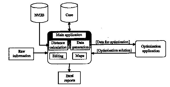
Figure 9. Overview of the FlowOpt system.
Information about, for example, supply and demand is company specific and denoted "Raw information". Road information from the National Road database (NVDB) is used when distances are calculated. All information necessary for the analysis is stored in a separate database, denoted "Case". The optimization module is located in a separate application. All data generation for the model including decisions about filtering of variables are done in "Data generation". All data is then translated into a mathematical model by use of a set of input/output routines and the AMPL modeling language (see [7]). As a solver we make use of the Cplex-optimization system (see [8]). Results from the optimization module are then imported back into the main application where different report options are possible. Normally, the results are exported to Excel or further calculations are done in a database in order to analyze specific key figures. The results are also interpreted in the main application where the viewer chooses different wood flows to show in the GIS system. This makes it easy, for example, to view catchments areas for different industries. The flow is shown either with straight lines as the crow flies or with lines marking the exact route. The viewed wood flows can also be exported as shape files in order to make more advanced presentations in commercial GIS tools.
The collection of data can be done in different ways, but normally data is collected from company databases. The system can either work with historical data or make prediction on future demand, supply and different train and truck capacities. This depends on the purpose of the analysis. Historical transportation data can be used to compare with an optimized solution of the same historical data. Prediction of future demand and supply is needed to optimize the future wood flow and, for example, the integration between truck and train.
Road Data Base
Digital, nation-wide road information represents a fundamental piece in the development of decision support systems in transportation. The Swedish National Road database (NVDB) was developed in a collaboration between the Swedish National Road Administration, the Central Office of the National Land Survey, the Swedish Association of Local Authorities and the forest industry.
For any given user of national road database it is important that data is up-to-date. This is handled through data registration at source i.e. the road manager is responsible for supplying data within its fields of operations. In this way data is registered by a manager with knowledge of the conditions and can ensure continued updating. The database contains digital information on all Swedish roads; the state road network, the municipal road and street network and private road networks. All roads, approximately over 500,000 km, are described geometrically, topologically and with detailed information about each road segment. This include road manager, road classification, road designation, height restrictions, load bearing obstacles, surface material, width and traffic regulations. For transportation on forest roads there are also special details about accessibility, turning radius, barrier etc. An illustration of the geographical information is given in Figure 10.
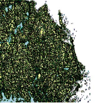
Figure 10. The Swedish National Road Database includes all Swedish roads. Here an illustration of the network around the city of Uppsala.
To calculate the actual driven distance between two locations is not straightforward. The transport agreements are typically not based on the shortest distance. Instead it depends on a combination of distance, speed limits, road owner, road width and road surface. In the system we can choose a combination of these factors in order to establish a distance table between all pairs of nodes used in the planning process. In practice, we choose a weighting for each attribute that are combined into a single value for each road segment. Those calculations are done in a separate function in the main application. In order to make the shortest path computation quick a special network is constructed based on the information from NVDB.
Solution Methods
The LP-problem without back-haulage variables is relatively easy to solve with a standard LPsolver. However, when back-haulage routes are to be used in the analysis we get too many variables to generate explicitly in the model. We call the model with explicit variables the Master problem. Initially we solve the problem with the set RB = Ø. In order to solve the overall problem we apply a solution strategy described in Figure 11. This is often referred to as column generation and is a well known method for solving large scale LP-models, see for example Nemhauser andWolsey (1988). To generate new variables or columns we need to solve a so-called Subproblem. The structure of the subproblem depends on the actual application. In our case we need to solve a constrained shortest path problem. The constraint is a limit on the length, in time, of the back-haulage route and represents the shift length of a truck driver, for example, ten hours.
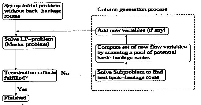
Figure 11. Overall solution procedure.
The subproblem is to find the best possible back-haulage route given the current LP-solution. More technically this means the potential variable (based on a back-haulage route) which has the most negative reduced cost. We set up a network where the arc costs are decided by the values of the dual variables from the Master problem. In the network we take into consideration all pre-processing available in order to limit the size of the network. There are several solution procedures and we have selected to formulate it as an integer programming network problem. The result from the Subproblem is translated into one variable defined by a physical back-haulage route and its composition with respect to assortment and assortment group (i.e. a new variable xkijhga). We only generate one variable in each Subproblem and this is too slow in practice. To overcome this we apply a pre-process and generate a large set of potential routes into a pool. Once we have found the best possible route from the Subproblem we search through the pool and generate additional variables which have a reduced cost below a particular threshold value (based on the solution from the Subproblem). The generation of variables in each iteration will stop either when the entire pool of pre-generated back-haulage routes have been examined or when a maximum number of variables have been added to the Master problem (we have used 1-2,000 as a limit). The overall algorithm is terminated either when a given number of subproblems are solved or when no negative reduced cost can be found in the subproblem.
CASE STUDY
We have used FlowOpt in several case studies and here we report on two of these. The first is about integration between truck and train transportation, and the second is about wood bartering between two companies. Both are based on real cases and due to confidentiality we cannot reveal the actual savings in monetary terms.
Wood Flow Integrating Truck and Train Transportation
Sveaskog is a forestry company responsible for 4,6 million hectares of forests of which 3,5 millions are productive. This corresponds to 16% of Sweden's total productive area. Sveaskog was to make a strategic decision about a new train system. This includes long term rental of train capacity (wagons and locomotives) and establishment of new terminals. Currently Sveaskog is using a train system called Trätåget ( eng. The wood train) to move wood from the northern part to the middle part of Sweden. In this case study a number of scenarios were investigated where an additional train system called Bergslagspendeln (eng. Pendulum of Bergslagen) is used to move wood from the central/south part of Sweden to the east coast in the middle of Sweden. Other wood assortments can be transported in the other direction. The new system also includes a number of potential terminals. Figure 12 illustrate the location of terminals together with supply areas and industries used in the study.
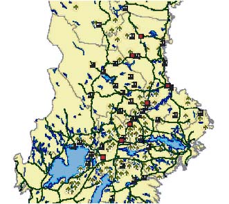
Figure 12. Overview of train network (solid lines), terminals (squares) sources (arrows) and industries (factories) used in the case study for Sveaskog.
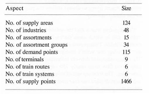
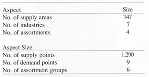
Five scenarios were set up. Each scenario involved a set of terminals, a set of train routes (for the given terminals) and particular capacities at both train systems and terminals. Each route has a capacity depending on how many times it runs every week and at which terminals it stops for loading and/or unloading. The cost of the train system relates to a fixed annual fee to use locomotives and wagons, terminal capacity and handling costs, and a volume related cost (i.e. number of wagons needed) depending on the volume transported. The difficulty in deciding about the new system is to evaluate its consequences in the entire transportation plan. It is, for example, important to compute any savings by entire transportation plans with the new train system. It was decided to collect information about supply and demand during the previous year and the study the impact if a new train system was used. Data about the actual case is given in Table 1.
Table 1. Data about the case at Sveaskog.
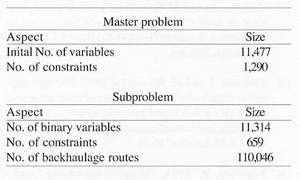
The optimization problem is summarized in Table 2. The number of potential number of backhaulage routes is the number generated for the pool. In this case this is based on an efficiency of 90% (i.e. saved unloaded distance is at least 10% of the overall distance). We can note that this is the number of physical back-haulage routes. The number of potential variables are larger as there are many combinations of assortments and assortment groups for each route in the pool. The time to solve the Master problem is about one minute. To solve and generate new columns takes about 10 minutes for each iteration. Most time is spent in setting up the integer network formulation and computing all arc costs. In each iteration we generate up to 1,000 new variables. In Figure 13 we show how the objective value changes with the number of column generation iterations for two scenarios. We have not addedthe fixed cost for the train system in the figure. A typical result for all case studies is that the impact of back-haulage routes is less when train systems are used. Many of the very efficient back-haulage trips over long distances are simply replaced by more efficient train transportation. In this case the savings using backhaulage routes is about 4% with train system and 7% without train system. In Figure 14 we show, for the same two scenarios, how many variables that are added in the solution process.
Table 2. Data about the optimization models at Sveaskog.
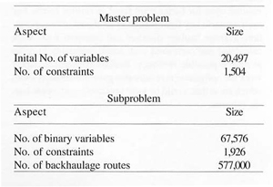
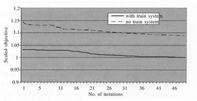
Figure 13. Scaled objective function value for two scenarios, one with and one without train system. The fixed cost for train system is not included.
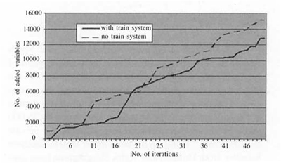
Figure 14. Number of added columns for two scenarios, one with and one without train system.
With the optimization we could quickly find optimal truck and train flow, train usage, terminal usage, train capacities, back-haulage possibilities and different import possibilities. FlowOpt was flexible and we could in short time establish maps and reports to illustrate the plans for further studies. Figure 15 illustrates the catchment area for one industry and one product when only trucks are used (left part) and when trucks and the Bergslagspendelnare used (right part).
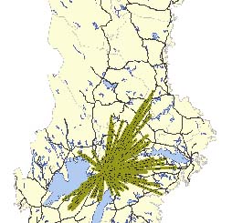
Figure 15. Catchment areas for one industry and one assortment group. Left part is with trucks only and right part with trucks and train.
The result provided valuable and critical information in the negotiations between the company and the train service provider. Using trucks and the Bergslagspendeln proved substantial gains in terms of systems efficiency. With the Bergslagspendeln the use of truck transports could be reduced by 35% reducing overall energy consumption by approximately 20%. Whether the industries. Bergslagspendeln will provide a reduced business cost or not depends on the needed increase in fixed costs, train capacity and infrastructure investments. These aspects are currently being evaluated.
Potential For Pulp Wood Barter
The two forest companies Holmen Skog and Södra Skogsägarna wanted to investigate the possible gains of enlarged pulp wood barter. Holmen Skog is one of the larger forest companies in Sweden and owner of over one million hectares of productive forests. Södra Skogsägarna is a co-operative economic association owned by 35,000 private forest owners. In total the estates of the private owners cover 2,1 million hectares forest land in southern Sweden. Both Holmen and Södra Skogsägarna have supply agreements with several pulp industries in the area, located in south east of Sweden. The companies produce the same assortments and barter a certain amount of pulp wood every month. In order to cut transportation costs Holmen Skog delivers pulp wood to industries where Södra Skogsägarna have a supply agreement and vice versa. Normally they barter the same amount of volume of a certain assortment trying to always deliver the pulpwood to the closest industry.
The objective was to find the optimal amount of barter volume and in which areas the exchange would be the most profitable. Transportation data from the two companies covering one yeart's transportation was collected. The data consisted of delivery information with the actual pulp wood flow from nearly 750 supply areas to seven industries. The total amount of volume was three million cubic meters divided into four quarters of a year. Data for the case is given in Table 3.
Table 3. Data about the case at Holmen Skog and Södra Skogsägarna.
The optimization problems are summarized in Table 4. The time to solve the Master problem is about one minute, and for the Subproblem about 5 minutes. In this case, there are not so many back-haulage possibilities as there are relatively few assortment and industries. Since not all assortments were included in the case study, results with back-hauling was not regarded so interesting in this particular case.
Table 4. Data about the optimization models at Holmen Skog and Södra Skogsägarna.
In the case study, several different scenarios were investigated and the total cost of transportation and barter volumes were compared to the actual transports during the analyzed period. The different scenarios treated various barter schemes e.g. no limits of barter - no barter possible for deliveries to specific industries - the amount of volume open for barter were fixed at various levels. For each scenario key figures such as total cost of transportation, average haulage distance and transport work were calculated and compared with actual transports in order to decide possible revenues. Besides cost and transport work the optimization results also gave information about which areas that would be most profitable to increase barter volumes.
Using the FlowOpt system we could quickly find the most cost-efficient truck flow with the optimization module and easily interpret the results in the main application. Best result showed the scenario in which there were no limits for pulp wood barter. In that scenario the optimum barter volume was about twice as big as the actual barter volume. The potential cost reductions where estimated to about five percent, caused by shorter haulage distance and less transport work. Less transport work will also reduce negative environmental influence from trucks. Figure 16 illustrates a conceptual picture of the difference in catchments areas for four industries without and with optimal barter volume. Crossing flow lines (as in the left part) indicate non-optimal flows.
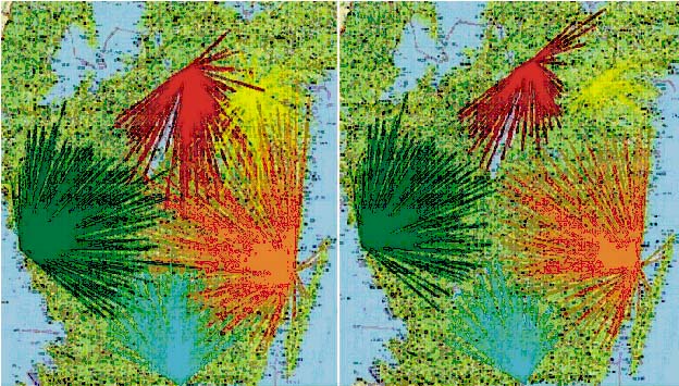
Figure 16. Catchment areas (illustrated by flows) for four industries owned by two different companies. The left figure shows no barter between the two companies and the right figure shows optimal barter.
CONCLUDING REMARKS
FlowOpt makes it much more efficient to perform case studies as compared to earlier semimanual systems. This is true both in terms of time to find an overall and integrated transportation plan and in the solution quality of the integrated planning. Flowopt will be a key instrument in future case studies. The optimization models are very flexible and robust and can easily adopt new restrictions and possibilities. The use of the road data base NVDB is also a critical tool of the system.
In FlowOpt we have chosen not to use binary variables to represent the usage of train systems or terminals. The main reason is that each combination of train capacity and terminal capacity and usage is based on detailed negotiations between the forest company and train service provider. In practice it is not possible to collect information on a general case as there are too many possible combinations. We therefore define one model for each case negotiated as companies, in general, only consider a very limited number of potential cases. Moreover, having a LPmodel makes it possible to get a correct sensitivity analysis.
Transport planning in Swedish forestry today is decentralized and manual to a high degree. Haulage in different forest-management districts is planned in each district by independent transport managers, and the transportation is carried out independently of those in other districts. The main drawback is the lack of coordination and possible redirections of flows, integration between trucks and trains or use of back-hauling are difficult to accomplish. In order to facilitate this efficient integrated planning the planning activities have to be supported by systems like FlowOpt. Several modules of the FlowOpot can be used to develop future company specific support systems. To use the model on annual planning is straight forward. In cases where shorter periods, for example one month, are used it is important to consider when supply become available and several time periods may be needed.
ACKNOWLEDGMENT
We thank the Swedish Agency for Innovation System for funding the project. We are also grateful for participating companies Optimal Solutions, Dianthus, Stora Enso, SCA, Södra Skogsägarna, Holmen Skog and Sveaskog.
AUTHOR CONTRACT
Mikael Rönnqvisty can be contacted by e-mail at --
miron@mai.liu.se
REFERENCES
[1] Carlsson, D. and M. Rönnqvist. 1998. Tactical planning of forestry transportation with respect to backhauling, Report LiTH-MAI-R-1998-18, Linköping University, Sweden.
[2] Eriksson, J. and M. Rönnqvist. 2003. Decision support system/tools: Transportation and route planning: Åkarweb - a web based planning system", Proceedings of the 2nd Forest Engineering Conference, Växjö, May 12-15, Sweden, 48-57.
[3] Forsberg, M. 2003. Transportsamordning Nord - Analys av returtransporter, Report nr 529 - 2003, Skogforsk, Uppsala, Sweden. (in Swedish).
[4] Martell, D.L., E.A. Gunn, and A. Weintraub. 1998. Forest management challenges for operational researchers, European Journal of Operational Research 104, 1-17.
[5] Rönnqvist, M., 2003, Optimization in forestry, Mathematical Programming Ser. B 97, 267-284.
[6] Nemhauser, G.L. and L.A. Wolsey. 1998. Integer and Combinatorial Optimization (John Wiley & Sons).
[7] Fourer, R., D.M. Gay, and B.W. Kernighan. 2003. AMPL _ A modeling language for mathematical programming, 2nd edition, (Thomson).
[8] ILOG CPLEX 8.0, User's manual, 2002.