Vol. 16, No. 2 July 2005
Dag Fjeld
Swedish University of Agricultural Sciences
Umeå, Sweden
Caisa Hedlinger
SCA Containerboard Nordic
Obbola, Sweden
The authors are, respectively, University Lecturer, Department of Silviculture, Swedish University of Agricultural Science, and Sales Coordinator, SCA Containerboard Nordic.
ABSTRACT
This paper presents the transport game; a pedagogical tool developed to provide a competition-driven introduction to important issues in transport planning. The competitive element of the game concerns minimizing transportaton. The game is played between three two-player teams. Each team has wood supply responsibility for a pulp mill and a saw mill. Given a varying weekly demand for each mill, the teams procure round wood from the 64 supply nodes in the region. The planning decisions in the game are aimed at minimizing the total transport distance (loaded + unloaded) for the weekly demand. Planning decisions have the following priority: 1) filling the mill demand, 2) minimizing the loaded transport distance by purchasing wood close to the mill 3) minimizing the unloaded transport distance by identifying backhauls flows.
The game forces the players to manually handle a high number of decision alternatives without any form of decision support. It is used to give the students a practical understanding of basic issues to accompany their theoretical lessons. It can also be used as an experimental laboratory to examine the effect of different restrictions on proficiency. The paper presents results from student exercises where development of player proficiency is examined.
Keywords: planning decision, complexity, cooperation, network.
INTRODUCTION
The focus of forest operations research and development in the Nordic countries has changed during the last decade. Earlier development has been dominated by the aim of cost minimization through rationalisation of labour, capital and finally, knowledge. Now development is also aiming at increasing the control and adaptability of forest operations involved in wood supply. With structural changes driving towards fewer and larger mills, transport issues are now emerging as key areas of knowledge for newly educated foresters.
The present annual education of MSc-level foresters in Sweden is 80 per year. With an annual harvest of approximately 80 million m3, the number of potential recruits is approximately one per million m3. These individuals are expected to handle a wider range of issues than earlier. While the use of management information systems, expert systems and advanced decision support are increasing, these still rely on a good understanding of basic issues.
Transportation in Forestry Education
An effective wood supply process is based on a hierarchy of planning sub-processes. Long term prognosis-based plans are revised in rolling supply/demand plans and confirmed in delivery plans. Delivery plans are then the basis for operational planning of both harvesting and transport. Transportation issues, however, have implications at many levels. The choice of transport systems has consequences for mill economies of scale and consumption volumes (strategic planning). Consumption volumes are determinants for the size of supply areas and average transport distances (tactical planning). The spatial distribution of supply areas determines the possibility for backhauls during truck routing (operational planning). As the final sub-process in wood supply, transport is the critical link where delivery obligations must be fulfilled with a high degree of precision.
In Sweden, much wood flow planning and vehicle routing in round wood transport is still done manually [12]. In forestry education, students completing elective courses in wood supply are expected to be familiar with basic principles and models for planning, execution and control as well methods for optimized decision support at each level. Transport issues are learned with a "top-down" approach starting with long-term issues and progressing to short-term operational decisions. Solving problems of optimal supply areas through exercises with MS EXCEL Solver optimization is not difficult. The number of decision alternatives in operational planning, however, is higher. Identifying potential routes and backhauls from the divergent flow of CTL assortments is a spatial problem of greater difficulty than originally perceived by the student. Specifying the necessary restrictions for real operations and need for heuristics to reduce problem size are important aspects to understand if students expect to participate in development projects after graduation. Most of these issues also have spatial aspects which are helpful to understand before beginning work with optimization solutions.
Goal
The aim of this paper is to present the principles and typical results of the Transport Game - a teaching tool used to provide students with an introduction transport planning in a cut-to-length (CTL) contest.
METHOD - THE TRANSPORT GAME
Gaming is an approach which has been used earlier as successful tools in logistics teaching. The Wood Supply Game [5, 8] for example, was developed from a popular teaching tool called the Beer Distribution Game [15] to give a more sector-specific example of demand distortion. The Transport game has been developed over a period of two years through regular use and feed-back in program courses. Two characteristics have been seen as important goals in its development. The first is that the playing environment should provide a high level of motivation for players. The second is that the exercise should be simple enough to be handled mentally without the need for mathematical support. Post-game calculations and reporting should also be simple, not requiring more than a pencil and paper.
The exercise in its present form requires 2.5 hours. Two hours are spent playing and a half an hour is spent on post-game calculations and discussion. Each individual game requires three two-person teams who compete during three "weeks" of wood supply. Each of the three teams has wood supply responsibility for one pulp mill and one saw mill. With larger groups a number of six-player games are played simultaneously.
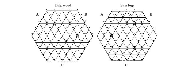
The game is played around a hexagonal wood supply region with 64 nodes supplying pulpwood and saw logs to six demand nodes (three pulp mills and three saw mills). The playing board has two identical maps, one for saw log supply to saw mills and one for pulp log supply to pulp mills. The volume of supply is expressed as the number of supply nodes. The actions of all teams are marked with whiteboard pens on the game board, which has an erasable plastic surface.
The goal for each team is to minimize the total (loaded and unloaded) transport distance for the three week playing period. Decisions have the following priority of goals:
1) Filling the exact weekly mill demand (mandatory)
2) Minimizing the loaded transport distance by purchasing wood close to the mill
3) Minimizing the unloaded transport distance by identifying backhauls flows.
Figure 1. The basic maps used in the transport game. The transport network is represented by the links which intersect at numbered supply nodes (1-64). The grey and black dots represent pulp and saw mills (demand nodes), respectively. The letters indicate the team (A, B, C).
Every week of play starts with the assignment of a weekly demand volume (expressed in nodes) per mill. Each team is then allowed to fill its mill demand by claiming the necessary number of pulp wood and saw log supply nodes on the respective maps. This is done according to a weekly randomly assigned sequence between teams. Claimed nodes are marked with team-specific colours of whiteboard markers. An example of the claimed nodes for one week's supply of respective assortments is shown below (Figure 2).
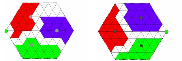
Figure 2. An example of one week's distribution of wood supply nodes between pulp mills (left) and saw mills (right). The nodes claimed by each team are marked by the shaded areas (team A: upper left, team B: upper right and team C: lower). The 3 grey and 3 black dots in the central areas represent the pulp and saw mills, respectively. If total demand exceeds total supply, wood may be imported (at a cost of 5.5 links).
Distances are measured by the number of links between forest and mill. The next step of the game is locating backhauls that minimize the unloaded transport back to the forest. Before starting the game a number of typical backhauls are demonstrated and their savings calculated. Three of these are shown below (Figure 3). Two adjacent mills using different assortments allows ample opportunity to find backhauls. Each backhaul, however, must be drawn on the map from its start point (a mill) together with the unloaded and unloaded path to prove its validity. The players are allowed to cooperate within and between teams. In the case of cooperation between teams, an equitable division of savings must be agreed upon before a backhaul may be recorded. This stage of the game is subject to a time limit.
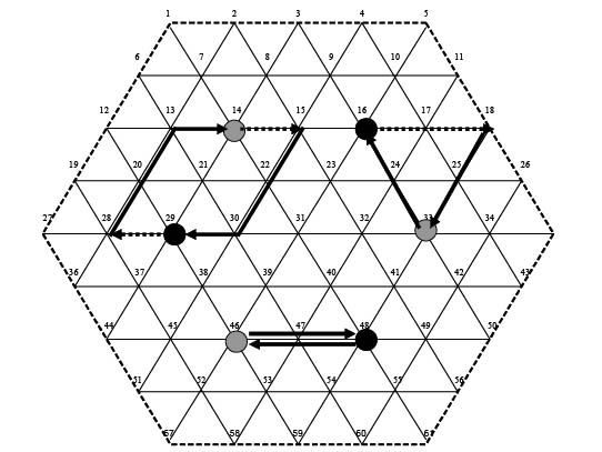
Figure 3. Three examples of backhaul flows between pulp mills (grey nodes) and saw mills (black nodes). The unloaded and loaded and transport distances are shown by the dotted and solid arrows, respectively. Both the upper left and lower backhaul save two links of unloaded transport per mill. The upper right backhaul saves one link of unloaded transport per mill.
After each week the final results are recorded on separate score cards and the game board is erased. After three weeks the results are calculated. The winning team is determined by which team has the least driven distance. First the theoretical driven distance is found by doubling the loaded driven distance between supply and demand nodes. From this, the backhaul savings of unloaded distance is subtracted to get the actual driven distance
Actual driven distance per team =
2  LDijk -
  SUDijk
LDijk = loaded distance (links)
SUDijk = saved unloaded distance (links)
for each week (i=1,2,3) and mill type (j=1,2) from each supply node (k=1…64)
Two variables are important in the post-game discussion of player decision proficiency. The first is the average loaded transport distance per unit of wood supply. This is a variable indicating proficiency at the tactical level which is calculated by dividing the sum loaded distance with the sum volume (nodes) of wood supply.
Average transport distance per team =
 LDijk / Nij
Nij = total volume of wood supply (nodes) for three weeks per team
for each week (i=1,2,3) and mill (j=1,2) from each supply node (k=1…64)
The second is the relative backhaul savings. This indicates proficiency in the operational level and is calculated as the ratio between the backhaul savings and the theoretical driven distance.
Relative backhaul savings per team =
 SUDijk / 2
  LDijk
LDijk
RESULTS OF STUDENT EXERCISES
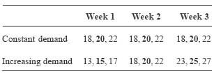
The game has been played under different game conditions. The factor which has the greatest influence on transport distance is weekly demand. Demand varies between weeks and teams. Two patterns of demand variation between weeks have been used. The first pattern is where the demand increases each week (first week: 15, second week: 20, third week 25). The second is where the general level is the same for all three weeks (20). In addition to the variation between weeks, a small degree of variation (+/- 2) is randomly assigned to the different teams (Table 1). The key variables from the student results may be examined under the game assumptions to see how these assumptions influence the development of proficiency.
Table 1. Typical demand patterns (nodes/week) for the transport game. For each week the alternative demand levels for each of the three teams is shown.
The main variable indicating proficiency at the tactical level is the average (loaded) transport distance (links/node). Figure 4 shows all the observed values collected within the current game version for varying demand levels.
A lower theoretical limit for weekly average (loaded) transport distance is calculated for each level of weekly demand (Table 2). Comparing the average transport distance to the minimum transport distance shows that the student teams transported round wood approximately 30 % farther than theoretically necessary. This extra distance increased with increasing demand.
Table 2. Minimum transport distances (loaded links/node) as well as the ratio between average and minimum transport distances for alternative demand levels (nodes/week).
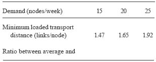

Figure 4. The average transport distance (loaded links/node) for a wide range of weekly wood demand (nodes/week).
Another perspective on the competition for supply nodes may be expressed in terms of factor market share (Figure 5). The games with constant demand have a higher market share at short distances and a lower market share at long distances than the games with increasing demand.
The main factor indicating proficiency at the operational level is the relative backhaul savings. This is the factor where a marked improvement in student proficiency was expected during the game. The development of weekly backhaul savings for both patterns of demand variation are shown below (Table 3).
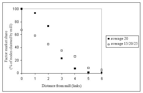
Figure 5. The variation in factor market share (proportion of wood supply bought by the mill) with increasing transport distance for games with constant (20) and increasing demand (15/20/25).
Table 3. The relative backhaul savings for each team and week of the student game. The backhaul frequency and savings per backhaul is also shown.
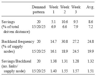
The results show that the average backhaul savings (measured in terms of % of total driven distance loaded and unloaded) increased with week number for patterns of both constant and increasing demand. For constant demand the increase was greatest between the first and second week. For increasing demand the increase was greatest between the second and third week. The same trends concern the frequency of backhauls. While the frequency of backhauls was greatest for constant demand, the savings per backhaul was greater for the increasing demand.
DEVELOPING STUDENT PROFICIENCY
The best direct measure of tactical proficiency in the game is the ratio between the average transport distance and the minimum theoretical transport distance (Table 2). The average ratio in this game was approximately 1.3. This is primarily a result of gaming between teams for control over the most suitable supply nodes. In most cases the students have tried to focus their claimed nodes in a roughly circular supply area, thereby minimizing the loaded transport distance. However, two factors have disturbed the formation of geometrically perfect supply areas. The first is the sequence that the teams were assigned for claiming nodes. The second is the total demand levels in relation to available supply nodes. The teams that are assigned first choice could establish geometrically perfect supply areas. The remaining teams had to adapt their supply areas to the nodes left over from the previous teams. The interdependence of supply areas is a point quickly picked up by students. Theoretical issues of supply area geometry to accompany the exercise (planar models) are covered by Sundberg and Silversides [16], Fohlin and Silver [6] as well as Haartveit and Fjeld [7]. The observed patterns for factor market share within different distances of the mill (Figure 5) can also be compared to Haartveit and Fjeld [7] and applied in conjunction with basic concepts of transport geometry in Sundberg and Silversides [16].
The second factor of importance for tactical proficiency is the total mill demand in relation to the available supply. When remaining nodes are scarce, this gives the last team an inefficient distribution of supply nodes and forces them to "import" at a high penalty (transport distance of 5.5 links/node with no chance for backhauls). In the games with constant demand, "import" represented only 0.3 % of the total demand. In the games with increasing demand, import represented 7-8 % of the total demand. In these cases, demand volumes in the final week sum to 75 nodes, exceeding supply by 11 nodes (18 %). Distributing the theoretical 18 % deficit over three weeks should yield an average of 6 %. This figure, however, is slightly lower than the actual results (7-8 %) , indicating that some of the teams have chosen to import at a distance of 5.5 links rather than accept "left-over" nodes at a distance of 6 links.
The development of operational proficiency is probably the most interesting aspect of the exercise. In both patterns of demand, backhaul savings have increased from week one to three (Table 3). The level of savings achieved by the students can be compared to the maximum limit which is possible under specific conditions in the exercise. For a demand of 20 nodes per mill and a near-circular supply area, 4 standard backhauls are possible. These four backhauls between the team's mills will enable a total savings per mill of 6 links (unloaded) for a total transport distance (loaded plus unloaded) of 65 links. Using the same logic, the upper proficiency limits for demand levels of 18, 20 and 22 nodes are 9, 10 and 13 % savings, respectively. These upper limits assume that the teams have circular supply areas (which minimize the loaded transport distance). From the results we see that the students are apparently attaining the maximum limit of proficiency already in the second and third week. The reason for this, however, is that many have chosen an oval supply area (with the longest axis aiming at a cooperating mill) instead of circular supply area. This makes it possible to increase the measure of operational proficiency (backhaul savings) but at the cost of decreased tactical proficiency (increasing the average loaded distance).
In the games with increasing demand the students achieved their highest proficiency in the third week (savings of 7-8%). In these games the variation in demand levels forces the student to allocate a higher proportion of attention to handling wood procurement delegations than transport efficiency. The greater variation in supply areas also increases the potential variety of backhaul alternatives, increasing the amount of spatial information which must be processed in order to identifying these. However, as seen in Table 3, the weeks with largest demand also provide opportunities for longer backhauls with greater savings.
CONCLUDING REMARKS
The transport game gives a unique opportunity to experience many aspects of wood supply, within a simple framework. The game integrates competition for suitable supply areas with negotiations for collective advantages. The most important lesson, however, is the development of proficiency in solving spatial problems. When first confronted with assortment-specific maps of wood flow, many students find the number of "unknowns" and degree of spatial complexity overwhelming. However by the end of the exercise, most have found mental routines for handling the number of the potential alternatives and identifying competitive solutions. The present version of the game has been based on between 2 and 4 "weeks". Most students identify the search for backhauls over two maps as the most difficult part. Many say that 3 weeks is still not enough to master the game. The present version has been subject to two external evaluations and is currently being revised to increase user-friendliness.
The experiences of the game can be used as a frame of reference to introduce important theoretical concepts of planning, execution and control of logistics systems. After becoming familiar with basic concepts, the students will more readily appreciate the practical possibilities to improve efficiency in transport operations. Basic concepts related to handling complexity and coordination include Conant´s law of partitioning of information rates [4] and Beer's ideas of self-regulating subsystems [1] as presented by Hulten and Bolin [9]. Suitable references for introducing optimized planning of wood flow and vehicle routing include Bergdahl et al [2], Carlsson and Rönnqvist [3] and Palmgren [13]. After this material has been covered, aspects of necessary restrictions [11], control system structure [9], and mobile data systems [14] are suitable topics for further student work.
AUTHOR CONTACT
Dr. Fjeld can be contacted by e-mail at --
Dag.fjeld@ssko.slu.se
REFERENCES
[1] Beer, S. 1985. Diagnosing the system: for organizations. Wiley, Chichester.
[2] Bergdahl, A., A. Örtendahl, and D. Fjeld. 2003. The economic potential for optimal destination of roundwood in north Sweden _ effects of planning horizon and delivery precision. International Journal of Forest Engineering Vol. 14 No. 1: pp 81-88.
[3] Carlsson, D. and M. Rönnqvist. 1998. Tactical planning of forestry transportation with respect to backhauling. Lith-MAT-R-1998-13. 19pp.
[4] Conant, R.C. 1976. Laws of information which govern systems. In: Facets of system science Klir, G J (ed) Plenum. Pp 419-448.
[5] Fjeld, D. 2001. The wood supply game as an educational application for simulating industrial dynamics in the forest sector. In: Sjöström, K & L O Rask (eds.) 2001. Supply chain mangement for paper & timber industries. Proceeding from 2nd Symposium on logistics in Forest Sector. Växjö 2001: 241-252.
[6] Fohlin, Å. and M. Silver. 1997. Kvantitativa modeller för lokalisering av sågverk. Luleå Tekniska Universitet, Institutionen för Industriell ekonomi och samhållvetenskap. Licentiatuppsats 1997:42 . pp 43-59.
[7] Haartveit, E. and D. Fjeld. 2000. Interregional variations in transport net geometry _ an analysis of wood procurement areas for Norwegian sawmills. In: Sjöström, K (ed.) 2000. Logistics in the forest sector. Proceeding from 1st Symposium on logistics in Forest Sector. Helsinki 2000. pp 165-187.
[8] Haartveit, E and D. Fjeld. 2004. The wood supply game _ a logistics flight simulator for the forest sector. In: Juga, J (ed) 2003. NOFOMA 2003 Proceedings of the 15th annual conference for Nordic researchers in logistics. University of Oulo: 512-526.
[9] Hulten, L. and H. Bolin 2002. Information exchange and controllability in logistics. Working paper - Transport Research Institute, Stockholm. 17 pp.
[10] Linnainmaa, S., J. Savola, and O. Jokinen. 1994. EPO A knowledge based system for wood procurement management. Paper from the 7th Annual Conference on Artificial Intelligence, Montreal (1995): pp 107-113.
[11] Karanta, I, O. Jokinen, T. Mikkola, J. Savola, and C. Bounsaythip 2000. Requirements for a vehicle routing and scheduling system in timber transport. In: Sjöström, K (ed.) 2000. Proceedings from 1st World Symposium on Logistics in the forest sector. Timber Logistics Club. pp 235-251.
[12] Nilsson, B. 2004. Kartläggning av transportstyrning inom skogsbranschen i Sverige. Examensarbete. Studentuppsatser i skogsteknologi nr 70, 2004.
[13] Palmgren, M. 2001. An approach to log truck scheduling. In: Palmgren & Rönnkvist (eds). Logistik och optimering inom skogsindustrin. Workshop Åre 11-14 mars 2001. LiTH-MAT-R-2001-16: pp 95-106.
[14] Roscher, M., D. Fjeld, and T. Parklund. 2004. Spatial patterns of roundwood transport associated with mobile data systems in Sweden. International journal of forest engineering Vol 15 No 1:53-59.
[15] Sterman, J.D. 1984. Instructions for running the Beer Distributions Game D-3679, System Dynamics Group, MIT, E60-383, Cambridge, MA 02139.
[16] Sundberg, U. and C.R. Silversides 1988. Operational efficiency in forestry Volume 1: Analysis. Kluwer Academic Publishers, Dordrecht.