Vol. 15 No. 2, March 2004
Teijo Palander
Janne Väätäinen
Sanna Laukkanen
Jukka Malinen
University of Joensuu
Finland
The authors are, respectively, Senior Lecturer of Forest Technology at the Faculty of Foresty, University of Joensuu, Finland, and Researchers of the Finnish Academy.
ABSTRACT
This study introduces a support method to use in modeling backhauling. The method minimizes a truck's on-road driving while empty. The backhauling model is based on a commonly used timber transport allocation model. Here, this model is applied to a simulated energy-wood network. The resulting optimization provides two different delivery plans for two-way transportation: one with a constraint to minimize travel distances when empty and the other without this constraint. By applying the empty-route minimization method, the best return routes for trucks are determined beforehand with fewer alternatives then left to be solved by the backhauling model. The results prove that the method can be used to minimize empty-route driving, but further development of the empty-route minimization method is still needed before it can be used in combination with the optimization of backhauling. Therefore, the effects of empty-route minimization on the transportation distances with respect to stand and hauling alternatives are discussed. In addition, the possibility of increasing the profitability of transportation, through the use of the method to optimize energy-wood backhauling, is also discussed.
Keywords: Two-way transportation, backhauling, routing, empty loads, Finland.
INTRODUCTION
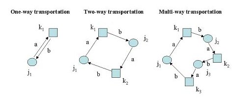
In Finland there has been increased discussion by transportation managers of wood procurement organizations about two-way or even multi-way transportation. However, one-way transportation is still characteristic of energy-wood transportation. This means that a truck normally carries a load to a destination then returns empty to the area where the load originated [2]. Long empty return routes usually increase transportation costs. Therefore various two-way or multi-way hauling models and methods have been developed to reduce empty vehicle movements for different transportation modes (Figure 1). Most of the models and methods are based on network theory or heuristics. This is why they are more or less similar in spite of what is transported or delivered.
In Finland and Sweden, backhauling models have been developed for timber transportation planning on a tactical level [2, 7, 8]. Backhauling means that a truck carries a load when returning from a destination to the area where the first load originated. In wood procurement, tactical planning consists principally of the allocation of wood flows from areas managed by regional procurement teams according to the demands of supra-regional mills, based on planning horizons ranging from a few days to a couple of months [6]. This planning process is at least supervised by a higher level of hierarchy in the procurement organization. Even though there have been problems with the practical application of backhauling models, the models have been used successfully to show the profitability of backhauling for wood procurement in Finland and Sweden.
Figure 1. Transportation modes: j1, j2, j3 = roadside inventories; k1, k2, k3 = power plants; a = distance driven with full loads; b = distance driven empty.
Some transportation models also include the minimization of empty-routes suggested as a solution to the empty vehicle allocation problem [7, 8, 9]. Empty-route minimization means that when trucks carry loads from one location to another the total distance the vehicle travels when empty is minimized. It is unclear why there has been little interest in developing optimization methods for empty-route minimization. A logical explanation may be that even though it is tempting to think of some great savings in transportation costs reached by any reduction in empty vehicle movements, the potential savings at present are minor for Nordic procurement organizations. This may also be the main reason why these optimization methods have not been applied to planning energy-wood transportation. At present, only Palander et al. [7] have presented a method to solve an operative timber transportation model with backhauling included.
The goal of this study was to develop a method that would include empty-route minimization, and then apply that method to two different simulated energy-wood networks to show its usefulness. Solving an operative backhauling model was also supported by the method. The effects of the method on empty movement were also determined. The conclusions were drawn up by comparing two modes of transportation: transportation with one-way loads and transportation with return loads. The comparison only considered the distance driven.
METHOD
The energy-wood transportation problem was solved by developing specific algorithms for inventory allocation modeling with backhauling and also for empty-route minimization. Conventional inventory allocation done by commonly used general allocation models does not effectively route trucks for backhauling. This conventional method does not provide users with information that is specific enough. A new routing algorithm was needed to determine any possible return loads for trucks from roadside inventories to power plants. The information about return loads was used in the backhauling model. The backhauling model was based on a simple linear programming (LP) model that is presented here without constraints [5]:
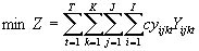 (1)
(1)
Where:
Z = optimum total costs ($),
Yijkt = volume (m3) of wood assortment delivered
from inventory j to mill k during period t,
wood procurement cost per unit volume
($/m3)
cyijkt = of wood assortment i delivered from
inventory j to mill k during period t,
T = number of discrete periods (two weeks)
of planning horizon,
K = number of mills,
J = number of inventories,
I = number of wood assortments.
The data was entered into the model via its LP matrix, which was in an American Standard Code for Information Interchange (ASCII) file format. The file was initially created as an information database using macro commands for Microsoft Excel software. The file was transformed and reformatted into an ASCII file: a manner specified by the Linear INteractive Discrete Optimizer (LINDO) program and contained parameter data in a form accessible by the LP model. This conversion also required the use of an in-house computer program written using Visual Basic language that read and formulated the file, inserting appropriate details or unit values for parameters not supplied by the Excel macros. After final conversion, the file needed only to be read and solved by LINDO. The backhauling model was as follows:
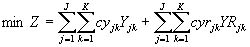 (2)
(2)
subjected to the following restrictions:
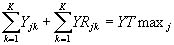
 (3)
(3)
non-negativity: Yjk, YRjk, ³ 0 (4)
Z = Optimum total cost ($),
Yjk = Volume
(m3) of energy-wood transported as one-way loads from inventory j to power plant k,
YRjk = Volume
(m3) of energy-wood transported as return loads from inventory j to power plant k,
cyjk = Transportation cost
($/m3) for one-way loads from inventory j to power plant k,
cyrjk = Transportation cost
($/m3) for return loads from inventory j to power plant k,
Dk = Volume
(m3) of energy-wood required at power plant k,
YTmaxj = Volume
(m3) of energy-wood that inventory j contains,
J = Number of inventories (1, …, j, …, 6),
K = Number of power plants (1, …, k, …, 4).
Both models were based on linear programming. It was therefore possible to rely on sound theory [3]. In the backhauling model two-way transportation was considered in the following ways. Volumes of energy-wood were the measurement unit for the transportation variables. In the models, the volumes were subjected to inventory constraints. After formulation of the backhauling model one possible return route for every one-way route was determined by a routing algorithm, which used a matrix technique for data handling. Two basic route matrices were produced consisting of data for one-way allocation. One matrix contained mill coordinates and another contained the coordinates for roadside inventories. Using these matrices the distances from roadside inventories to mills were determined in the first stage of the algorithm. After that, all possible return loads were determined for every one-way load. The shortest distance of travel for a backhaul route was used as the criterion for selection of the best return route. This method was assumed to minimize empty driving. The best return load for every one-way load was used by the backhauling model.
The core of the empty-route minimization method is its routing algorithm. Thus the method was tested on the energy-wood networks after routing of the return loads with the routing algorithm. The usefulness of the empty-route minimization method was evaluated by comparing the total distance in kilometers driven empty for one-way and two-way transportation. Transportation of energy-wood was assumed to use standard trucks normally utilized for pulpwood and saw timber transportation. The size of a load was therefore about 50 m3 and all energy-wood from the forest stands was delivered as bundles of logging residue.
MATERIALS
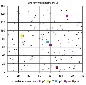
The empty-route minimization method was tested on two different simulated energy-wood networks. The areas of both networks were 22,400 km2 and each contained five different power plants (Figure 2). In the first energy-wood network the power plants were located in the same spatial pattern as the five largest power plants in the Finnish Province of North-Karelia. For the second energy-wood network the power plants were distributed in such a way that two-way transportation was assumed to be more profitable than for the first network. Distances between the inventories and the power plants were calculated from their x-,y-coordinates and multiplied by a road curving factor of 1.3 [8].
Figure 2. Two simulated energy-wood networks with the locations of the power plants (pp1, pp2, pp3, pp4 and pp5 = power plants).
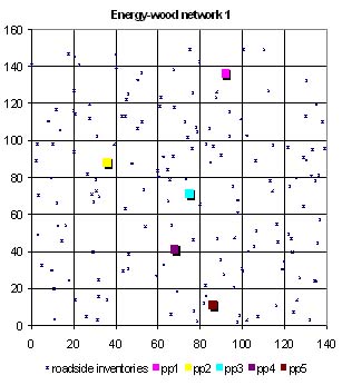
Roadside inventories of energy-wood were generated by Malinen and Palander [4] using forest stand simulator models. The inventories were then randomly located throughout the network area. All of the forest stands generated were pure pine that had been cut and hauled from the forest to form roadside inventories. The share of energy-wood on each stand was tested to be one of nine different energy-wood percentages, which varied from 12 to 20 percent of all the wood obtained from a stand. The energy-wood demands of the power plants were drawn from the potential yearly demands of the power plants situated in the Province of North-Karelia [1]. The demands of the power plants as well as the forest inventories were simulated for a one-week period (Tables 1 and 2). Wood procurement was assumed to be organized by one organization.
Table 1. Demands of the power plants for a one week period: k = demand of a power plant (m3).
| Power plants | k (1 week) |
| pp1 | 1250 |
| pp2 | 385 |
| pp3 | 1923 |
| pp4 | 135 |
| pp5 | 1538 |
| total | 5231 |
Table 2. Total amount of energy wood in roadside inventories as specified by the energy-wood percentage of the stands harvested.
| Energy-wood percent | Roadside inventories (m3) |
| 12 | 5514 |
| 13 | 6042 |
| 14 | 6582 |
| 15 | 7135 |
| 16 | 7702 |
| 17 | 8282 |
| 18 | 8876 |
| 19 | 9484 |
| 20 | 10108 |
RESULTS
Empty-Route Minimization
Some examples of the allocations of the return-routes by the empty-route minimization method are presented in Table 3. The method specified the roadside inventory from which a return load had to taken and the power plant where it had to be delivered. For example, if a one-way load was delivered from roadside inventory 1 to power plant 1 on energy-wood network 1, the return load was to be taken from roadside inventory 92 and delivered to power plant 5. The method seemed to indicate the same return routes for several different one-way loads. For example, on energy-wood network 1 the return routes were the same, if a one-way load was delivered from either roadside inventory 3 or 4 to any of the power plants. On energy-wood network 2 the method performed in a similar manner, but the results were different.
Table 3. Examples of the allocation of the return loads by the empty-route minimization method on energy-wood networks (ENs) 1 and 2: j = roadside inventory (RIs) from where the return load had to be picked up; k = power plant where it had to be delivered.
| ENs | RIs | Return routes (j, k) |
||||
| pp1 | pp2 | pp3 | pp4 | pp5 | ||
| 1 | 1 | 92, 5 | 73, 5 | 49, 5 | 49, 5 | 49, 4 |
| 2 | 30, 3 | 117, 1 | 30, 1 | 146, 1 | 92, 1 | |
| 3 | 30, 3 | 12, 3 | 132, 4 | 132, 3 | 49, 4 | |
| 4 | 30, 3 | 12, 3 | 132, 4 | 132, 3 | 49, 4 | |
| 2 | 1 | 138, 3 | 10, 4 | 73, 5 | 58, 5 | 58, 4 |
| 2 | 138, 3 | 111, 1 | 138, 1 | 141, 3 | 73, 3 | |
| 3 | 138, 3 | 90, 3 | 141, 4 | 141, 3 | 58, 4 | |
| 4 | 138, 3 | 90, 3 | 141, 4 | 141, 3 | 58, 4 | |
| 5 | 138, 3 | 90, 3 | 141, 4 | 141, 3 | 58, 4 | |
Backhauling Optimization
The amount of energy-wood as one-way loads, as return loads, transported in total, and the energy-wood share of the return loads according to the energy-wood percentages of the stands are presented in Table 4. The amount of the return loads seemed to increase at the same rate as the energy-wood percentage increased. The amount of return loads was highest when the energy-wood percent was highest. On the other hand the energy-wood share of the return loads increased until the energy-wood percent was sixteen, but started to decrease after that. However, the decrease was so small, only 0.1 of a percent, that the system seemed to be stable with respect to an increase of the energy-wood share.
Test of the Empty-Route Minimization Method
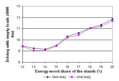
The distance driven empty did not decrease as was assumed when two-way transportation was used. On the contrary, more kilometers were driven empty for two-way transportation than for one-way transportation in spite of the energy-wood share (%) of the stands (Figure 3). However, the difference in the total distance driven empty between the transportation modes was not large.
Table 4. Amounts of energy-wood as one-way loads, as return loads, transported in total, and the energy-wood share of the return loads according to the energy-wood percents of the stands.
| Energy-wood (%) | One-way loads (m3) | Return loads (m3) | Total loads (m3) | Return (%) |
| 12 | 5456 | 68 | 5524 | 1,2 |
| 13 | 5902 | 136 | 6038 | 2,3 |
| 14 | 6432 | 127 | 6559 | 1,9 |
| 15 | 6971 | 158 | 7129 | 2,2 |
| 16 | 7529 | 175 | 7704 | 2,3 |
| 17 | 8094 | 186 | 8280 | 2,2 |
| 18 | 8634 | 236 | 8870 | 2,7 |
| 19 | 9225 | 249 | 9474 | 2,6 |
| 20 | 9838 | 264 | 10102 | 2,6 |
Figure 3. Kilometers driven empty for two-way and one-way transportation modes based on the energy-wood share (%) of the stands.
DISCUSSION
In previous studies of Finnish wood procurement, backhauling optimization and empty-route minimization have usually been treated separately [7, 8]. In this study empty-route minimization was used to reduce the decision alternatives for the backhauling model. In this way it is possible to solve larger models. In practice models may often be so large that they cannot be solved effectively without making compromises with the form of the models. The models may then tend to simplify the real world to such a great extent that the results do not satisfy the requirements of decision makers.
The empty-route minimization method seemed to give profitable return routes, in which the two-way return route distances were quite close to the one-way return routes distances. Because of the method the suggested return routes were the same for many different one-way routes. This was since the minimization of the empty travel distances on backhaul-routes focused the selection of the return routes to the same best choice inventories and power plants. This was probably the reason why the empty-route minimization method did not have great variability in the amount of empty driving for the transportation alternatives compared.
The backhauling model that was formulated together with the empty-route minimization method seemed to perform well, but the return loads did not include very large shares of energy-wood. This was probably due to a lack of timber assortments in the optimization [See also 8]. If the amount of pine logs and pulpwood for each stand had been considered in the optimization, the amount of the return loads would have been greater. Evidently, the energy-wood share of the return loads stabilized at a relatively low level for the same reason. More work may be needed to combine energy-wood and timber transportation networks.
Although the method for minimization of empty-routes and the model for optimization of backhauling were tested on energy-wood networks, the results would have probably been the same for any other wood procurement environment. This is partly due to the assumptions made in this study. It is notable that in real-world situations the energy-wood flow from forest areas to power plants is not as organized as it is assumed to be in this study. However, the purpose of this study was to develop a method to be used to minimize empty-route driving in combination with the optimization of backhauling. The results prove that at least the second objective was reached, but further development of the empty-route minimization method is still needed before the first objective can be reached.
In further studies the method and the model should be tested on environments that are more comparable to real-world wood procurement environments. Such studies should eventually prove the actual benefits of the method and the model. For different real-world applications, cost/benefit analysis is needed and even organizational changes may be needed before these new transportation modes of energy-wood transportation can be realized.
ACKNOWLEDGEMENTS
This study is a part of the "Group Decision Support in Wood Procurement" research project. The leader of the project is Docent Teijo Palander. Funding was provided by the Academy of Finland.
AUTHOR CONTACT
Teijo Palander can be contacted by email at:
teijo.palander@joensuu.fi
REFERENCES
[1] Asikainen A., T. Ranta, J. Laitila and J. Hämäläinen. 2001. Cost Factors and Large Scale Procurement of Logging Residue Chips. University of Joensuu. Faculty of Forestry. Research Notes 131. 107 pp.
[2] Carlsson, D. and M. Rönnqvist 1999. Wood flow problems in Swedish forestry, Skog Forsk. No 1. pp. 26-29.
[3] Hadley, G. 1964. Nonlinear and Dynamic Programming, Addison-Wesley Publishing Company. Inc., Reading, MA. 484 pp.
[4] Malinen, J. and T. Palander 2003. Artificial Marked Stands and Tree Generation for Wood Procurement Research Purposes. (Manuscript).
[5] Palander, T. 1997. A Local DLP-GIS-LP System for Geographically Decentralized Wood Procurement Planning and Decision Making. Silva Fennica 31(2):179-192.
[6] Palander, T. 1998. Tactical Models of Wood-Procurement Teams for Geographically Decentralized Group Decision Making, D.Sc. (Agr. and For.) thesis. University of Joensuu. 152 pp.
[7] Palander, T., J. Väätäinen, S. Laukkanen and P. Harstela 2002. Back-hauling Optimization Model for Finnish Wood Procurement. In: Conference Proceedings of Fourth International Meeting for Research in Logistics. de Carvalho, J. C. [Ed.] Lissabon, Portugal 2002. pp. 595-607.
[8] Väätäinen, J., T. Palander and P. Harstela 2002. Puunhankinnan meno-paluukulje-tusten optimoin-timalli. [A backhauling optimisation model for wood procurement.] Metsätieteen aikakauskirja 1:5-17. (In Finnish)
[9] http://www.storaenso.com. Accessed on 18. November 2003.