Vol. 14. No. 1 January 2003
Olivier R.M. Halleux
F & W Forestry Services
Albany, GA, USA
W. Dale Greene
University of Georgia
Athens, GA, USA
The authors are, respectively, GIS Specialist and Developer, F & W. Forestry Services, and Professor, University of Georgia.
ABSTRACT
Operational harvest planning in the southern USA has not been widely used in the past due to a lack of state legislation, non-regulatory water quality protection programs, and relatively easy logging conditions. Increased government regulation and market pressures to document sustainable forest management under various certification standards is increasing the need for harvest planning in the region, particularly on private, non-industrial timber sales. We developed an ArcView extension, Setting Analyst (SA), to assist harvest planners. SA can use spatial information obtained from scanned air photos or detailed data from a geographic information system. It models travel patterns of ground-based machines and compares different harvest settings based on projected average skidding distance, costs of skidding and improvements, and site disturbance levels. In its current form, it does not account for slope. SA can model settings with complex features such as stream crossings, restricted areas, and skidding on designated trails. Travel intensity is assessed since it is highly correlated with site disturbance and soil compaction. To assess the utility of SA, we used it to model ten actual harvesting settings and contrasted each with two proposed settings. SA produced sale plans that were very similar to those observed on the ground. Its primary advantage is that it conveniently documents each alternative setting considered for the timber sale. These can be kept on file to demonstrate the level of planning used when forest certification audits are conducted. SA offers the most potential to harvest planners that already use GIS or GPS but desire additional analysis and documentation capabilities.
Keywords: Operational harvest planning, GIS, average skidding distances, site disturbance.
INTRODUCTION
Operational harvest planning involves the design and organization of a timber harvesting operation and focuses on locating improvements such as roads, logging decks, skid trails, and stream crossings. The planner's objective is to find a procedure that balances economic efficiency with environmental considerations while ensuring legal compliance and minimizing potential safety hazards for all associated parties. The harvest planner may be a consulting forester who works for the landowner, a procurement forester who purchases the timber, or the logging contractor who actually performs the harvesting or combination of all of the above. The planning horizon influences the amount of information acquired and how the information is stored, for example, company land versus landowner assistance programs versus short term timber purchases. Information technologies such as global positioning systems (GPS), geographic information systems (GIS), and the Internet present new opportunities for collecting information pertinent to timber harvesting.
Harvest planning is common practice in many parts of North America and in other parts of the world. However, for various reasons formal harvest planning has been less widely used in the southern USA. The principle reason is the lack of regulations that require it. State forest practice acts are rare in the South. Most southern states employ non-regulatory Best Management Practices (BMPs) to protect water quality. The terrain in the South is relatively gentle, hence the planning required for cable or ground-based harvesting on steep terrain is not needed. In the Pacific Northwest, terrain is the key consideration whereas in the South it is usually soil and water. Non-industrial private timberlands provide a significant portion of the southern timber harvest, often from relatively small timber sales. This private ownership limits government influence on productive timberland. Finally, contractors, not company operated crews, perform essentially all timber harvesting.
Harvest planning will likely be increasingly important in the future as more environmental regulations are adopted and as the marketplace demands compliance with various certification schemes. Regulation of harvesting at the local or county level has increased rapidly in many states. Some local and county governments now require the submission of formal harvest plans to obtain a permit or approval to harvest timber in their jurisdictions. In addition, forest managers and contractors are increasingly expected to justify their decisions during third party audits for various forest certification programs. The Sustainable Forestry Initiative (SFI) illustrates the push by the forest industry to promote sustainable forestry and maintain an economically viable industry while satisfying the increasing demand for environmental responsibility [1]. Most certification standards require some form of harvest planning and documentation. Private and corporate landowners are concerned about site disturbance and damage during logging. As clearcuts get more complex in shape to meet aesthetics objectives, skid trail design will be increasingly important. Machine travel paths may be predetermined rather than simply evolving during skidding. As always, there will be an increasing push for economic efficiency and greater emphasis on reducing environmental impacts by either market or regulatory forces.
OBJECTIVE
The objective of this project was to develop a computer based harvest-planning tool that would allow the comparison of alternative harvest settings based on estimates of harvesting cost components and site disturbance. Our focus was to keep the model simple and use the information resources commonly available to forest managers, wood buyers, and logging contractors. The tool developed was not intended to derive the optimal mathematical solutions, but rather use simulation to allow comparisons between different user-defined harvest settings. This tool should be an aid to, not a replacement for, field-based harvest planning and should help improve the documentation of the planning procedures used. Finally, we wanted a technique that would work with commonly available software.
BACKGROUND
Estimating harvesting costs is a crucial component of harvest planning. The aim is to design an operation that will minimize road construction, logging deck construction, equipment setup, and skidding costs. Matthews [5] provide the early groundwork for harvesting cost analysis and inspired further development of the average skidding distance principle. Average skidding distance (ASD) is a variable that can be used in the cost analysis of a harvest plan. ASD is the average distance a machine must travel from felled wood to the logging deck for a particular setting. ASD can be used to estimate the total direct skidding cost.
Suddarth and Herrick [8] described a method to estimate ASD for irregular tract boundaries called the approximation method. This method forms the foundation of this research project, as it is consistent with raster or pixel-based GIS data structure. The horizontal area of the setting is divided into a finite number of mutually exclusive rectangles. The sum of the area-weighted distances from the logging deck to the geometric center of each rectangle divided by the total area of the setting gives an estimate of the ASD. As the number of subdividing rectangles approaches infinity, the calculation produces the exact average skidding distance.
Vehicle traffic during logging can cause soil compaction, rutting, loss of soil structure or other types of soil damage [2, 3, 6, 7]. Numerous studies over many years have shown that the number of machine passes over a piece of ground is highly correlated with site damage and that most damage occurs during the first five passes [7]. Tree growth and survival are influenced by soil properties, hence travel intensity or the number of passes through a particular area, is often a concern to foresters and harvest planners [2, 3]. Wang [9] found that no programs simulated harvesting systems from the standpoint of travel intensity and included it as a component of an interactive computer simulation program. He developed a travel intensity grid in which the pixel value was equal to the number of machine passes through the cell. Areas of high travel intensity could be used in conjunction with soil maps to compare skid trail configurations and identify a configuration with an acceptable level of compaction matched to soil types.
SETTING ANALYST
We named the tool we created as Setting Analyst. It functions within the ArcView GIS 3.2 environment. ArcView was selected for its popularity, cost, and capabilities. Setting Analyst estimates costs for skidding and improvements. Improvements include the cost of opening and closing features such as roads, logging decks, and skid trails. In addition, Setting Analyst highlights areas on the tract where the greatest machine travel will occur, thus identifying areas of potential soil compaction. The tool works as a simulation allowing the comparison of alternative user-defined scenarios. Setting Analyst is not an optimizer; rather it simulates using information provided by the user and lets the user decide the preferred setting. Setting Analyst assumes uniform timber density and does not consider slope at this time.
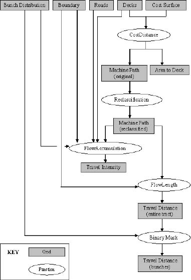
Setting Analyst was written in Avenue, ArcView's built-in object-oriented scripting language. The functionality contained in the scripts is packaged in the form of an ArcView extension or plug-in. We assumed users would have a basic working knowledge of ArcView and GIS to effectively use the tool. Setting Analyst relies on the Spatial Analyst extension, which allows the display, creation, manipulation, and analysis of grid or raster data. Setting Analyst uses existing functions to model machine travel in what is effectively a grid-based network analysis. Setting Analyst consists of two pull-down menus, two buttons, and three tool buttons. These are added to ArcView upon activating the extension. The model consists of a series of Spatial Analyst grid functions, reclassifications, binary masks, and grid manipulations. The user creates a cost or friction surface that controls the machine travel through the tract. The tool then uses the CostDistance function to generate a Machine Path grid based on this cost surface. The FlowAccumulation and FlowLength functions use this machine path grid to calculate travel distances and travel intensity. The interaction of these main functions is illustrated in a flow diagram found in Figure 1. The starting point is five grids of equal cell size and extent (grid dimensions). The user selects the appropriate tract, bunch distribution, roads, decks, and cost surface grids. The tract grid corresponds to the boundary of the harvest area. The bunch distribution grid represents a random distribution of log bunches. Decks and roads, as the name suggests, represent these features. The cost surface is a composite of feature grids and controls the machine travel directions.
The Cost Surface grid is the essence of Setting Analyst. A cost surface is a grid surface where the cell value is the cost-per-unit distance of passing through that cell. The CostDistance function selects the lowest cost path through the cost surface. Since low cost cells are preferred, we can control machine travel by assigning low cell values to skid trails and high cell values to restricted areas. For example, if the cost surface had a common cell value of 10 and a value of 5 where the skid trails were located, and 100 for a wet area, the trail will be preferred and the wet area avoided when selecting the least cost path through the surface.
While harvesting, the felling machine will make piles or bunches of logs in preparation for the skidding phase of the operation. Setting Analyst assumes that each bunch is removed with a single visit from the skidding machine. To simulate this situation in the form of a grid, a distribution of bunches is needed. The tool randomly generates a representative distribution of bunch locations based on the harvested timber tonnage per acre and the extraction machine's haul capacities. Each cell with a non-zero value represents a bunch. The machine travels to that cell to collect the logs and hauls them to the logging deck. Since the bunch distribution is randomly generated, this is a stochastic feature of the technique that introduces variation in the distribution and number of bunches. We considered this to be acceptable since this is a simulation and sampling methods to estimate timber volumes also provide estimates with variability.
The CostDistance function is used to determine the least cost path through the cost surface. The algorithm behind this function uses graph theory. This function creates a cost direction grid or what we have called the Machine Path grid. The cell values are in an eight-way direction code corresponding to the direction the machine will travel from the cell along the lowest cost path. A reclassified form of the grid is then used by the FlowAccumulation and FlowLength functions. The FlowAccumulation function generates the travel intensity grid that summarizes the number of machine passes through a cell. This function was originally a hydrological function that created a grid of the accumulated flow to each cell as rainfall in a catchment accumulated in streams then in rivers. In Setting Analyst, the machine "flows" through the cost surface and travel accumulates in low cost cells. The FlowLength function is also a hydrological function that calculates upstream or downstream distance along a flow path for each cell. In Setting Analyst this function calculates distance along the machine path for each cell. In the resulting grid, each cell value represents the distance from that cell to the nearest deck along the machine path. The grid is then masked by the Bunch Distribution grid so that only cells containing bunches remain. The average cell value of this grid is the average distance from all log bunches to the nearest logging deck or the ASD.
Deciding on an appropriate grid cell size was difficult. Cell size influences processing time and file size. . McDonald [6] used a 0.5m cell size for their GPS machine movement assessment, but they were trying to model tire locations. We started out using 10m and 1m cells. A 10m cell would over estimate the skid trail width and thus the area compacted. A 1-m grid size would underestimate the site disturbance. A skidder is roughly 3-4m wide and won't always move with the wheels in exactly the same place so 5m was a suitable compromise and is consistent with what Wang [9] used in his harvesting simulator
OPERATING PROCEDURE
The first stage of planning a harvesting operation is to conduct a field reconnaissance to get an understanding of site features and consider possible locations for logging decks, skid trails, stream crossings, and roads. Once back in the office, using ArcView the planner begins by creating shape files representing these features in potential locations. At least four methods are available to create shape files: digitized onscreen with a digital orthophoto background, digitized onscreen with a digital raster graphic (DRG) background, uploaded GPS data, or existing data sets (Figure 2). All the shape files are converted from a vector to raster (grid) data structure with a 5m (~ 0.25 chain) cell size.
Figure 1. Flow diagram of the Setting Analyst model.
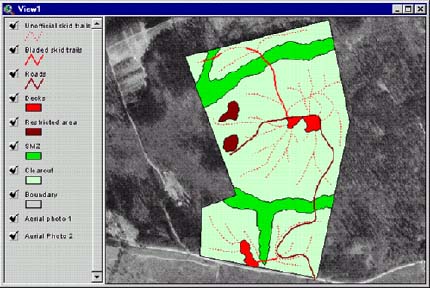
Figure 2. Setting features compiled from GPS data and by onscreen digitizing.
The next stage involves generating a random bunch distribution grid. The user enters machine payload (tonne/turn) and the number of tonnes of timber harvested per acre via the dialog box. Next, the user creates a cost surface to control machine travel through the tract. Selected feature grids are assigned weightings and then combined to form a composite or cost surface grid. The user can select from two cost surface generation approaches: merge and addition. The addition approach considers original cell values whereas the simpler merge approach does not. The cost surface is modified to incorporate stream crossings. The resulting cost surface restricts machine movement through the streamside management zone (SMZ) or riparian buffer forcing the machine to cross at designated locations. A further modification accounts for areas where machine travel is not permitted. Such areas might be ponds, areas excluded from harvesting, cliffs or existing high erosion. This forces the CostDistance algorithm to guide the machine around rather than through these areas. The user selects the appropriate boundary, deck, cost surface, bunch distribution, and road grids that make up the setting to be analyzed. The simulation is run and the resulting Machine Path, Travel Intensity, Travel Distance grids are added to the Setting Analyst Output view. The Summary Statistics function produces a summary report for the setting configuration. Overall tract ASD and the maximum skid distance are calculated. The Travel Intensity grid is reclassified in 0-1, 2-5, 6-20 and 21+ pass classes and the area in each travel intensity class is reported (Figure 3). Cost Calculator, the final stage of the analysis, uses previously generated statistics and user entries to calculate skidding cost, improvement cost, and total cost on a per tonne basis. The skidding cost per tonne is calculated using the following equation:
SC = (CPMH * CT) / (60 * PL) (1)
SC = per unit skidding cost ($/tonne)
CPMH = skidding cost per scheduled machine hour ($/hour)
UT = skidder utilization (%)
CT = skidder cycle time (minutes)
PL = skidder payload (tonnes)
The user can now repeat the analysis for alternative settings being considered and then compare the results. In comparisons discussed here, we assumed CSMH = $50, UT = 70%, and PL = 2.3 tonnes.
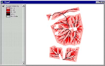
Figure 3. Travel intensity grid (number of additional machine passes through each cell).
FIELD TRIALS
Ten recently harvested tracts were modeled in an effort to further refine Setting Analyst and test its capabilities. For the purposes of this article one example will be illustrated. Notable features recorded by GPS used to create the actual harvest setting (Figure 4). Additional unimproved skid trails were subjectively added to direct the flow of machine traffic. In addition to the actual harvest settings two alternative settings were designed for each tract, modeled with Setting Analyst, and then contrasted with actual settings. The first setting type, "with existing roads", assumed that all the actual roads were present before harvest planning commenced (Figure 5). In this situation, the planner has the option to use the existing roads or not and simply locates decks and other additional features. This scenario often occurs where the tract is on industrial land with an existing road network. This setting type was designed with each deck servicing at least 8.1 hectares (20 acres). The second setting type, "without existing roads", assumed there were no or minimal existing roads (Figure 6). This setting type had fewer restrictions. The number of decks was of less concern, but truck stream crossings were avoided wherever possible in favor of temporary skidder crossings. A situation like this often occurs on non-industrial private lands. Similar weights were used to generate cost surfaces and approximate per unit costs were derived from various industry sources. The physical, travel intensity, and economic characteristics for each setting of the tract are illustrated in Table 1.
RESULTS
The goal of Setting Analyst is to provide additional information for harvest planners when they are considering alternative harvest setting configurations. The obvious question after modeling will be: Which is the best setting? It depends on how the planner prioritizes and reflects the operational issues on a given harvest unit. Is minimizing the number of stream crossings a major priority? Is cost paramount? Are longer skid distances and few logging decks acceptable despite the increased area with high travel intensity? The user determines the preferred setting, not the tool.
The settings designed with SA were very similar to those planned without it. This was not unexpected since SA was designed to assist, not replace, field-based harvest planning. The actual settings typically appeared well designed or very intuitive. Setting Analyst is not designed to generate the optimal solution, nor can it be assumed that current informal planning gives poor results. Current planning is simply not well documented. These tracts were on industry land where many roads already existed. Land management foresters, wood buyers, and loggers planned sales. Loggers were well trained in proper planning and harvesting techniques. Larger cost savings might be available on non-industrial private forestlands, especially if the logger is asked to do all planning and no foresters are involved or lead-time is short.
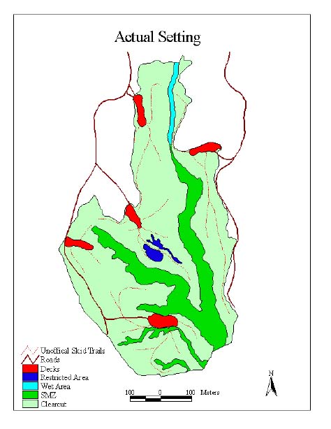
Figure 4. Actual harvesting setting based on GPS work.
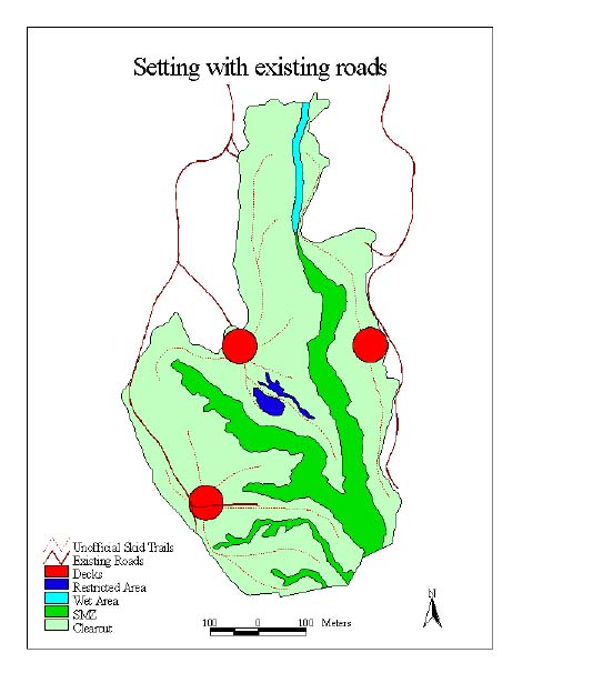
Figure 5. Harvesting setting with existing roads.
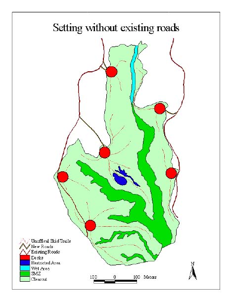
Figure 6. Harvesting setting without existing roads.
Table 1. Physical, travel intensity, and economic characteristics of the settings modeled.
| Setting Modeled |
|||
| Characteristic | Actual | With Existing Roads | Without Existing Roads |
| Physical Properties | |||
| Average Skidding Distance (m) | 131 | 175 | 115 |
| Maximum Skid Distance (m) | 671 | 585 | 390 |
| New Road Length (m) | 0 | 0 | 22 |
| Existing Road Length (m) | 3460 | 3460 | 2993 |
| Decks | 5 | 3 | 6 |
| Area Serviced per Deck (ha) | 5.5 | 9.1 | 4.6 |
| Area by Travel Intensity Class | |||
| 0-1 passes (ha) | 18.5 | 18.4 | 19.4 |
| 2-5 passes (ha) | 4.9 | 5.1 | 4.4 |
| 6-20 passes (ha) | 1.4 | 1.1 | 1.1 |
| 21+ passes (ha) | 1.1 | 1.3 | 1.1 |
| Setting Costs | |||
| Skidding ($/tonne) | 2.30 | 2.49 | 2.22 |
| Improvements ($/tonne) | 1.96 | 1.62 | 2.46 |
| Skidding + Improvements ($/tonne) | 4.26 | 4.11 | 4.68 |
| Skidding + Improvement ($) | 18,398 | 17,828 | 20,252 |
DISCUSSION
Field trial results
Modeling the ten recently harvested tracts suggests the model does have potential for use in planning timber sales. Further research is required to assess how harvesting costs derived by Setting Analyst correspond with those of the logger. A more hands-on approach to model verification could include using a GPS unit mounted on a skidder in an actual harvesting operation. For example, McDonald et al. [6] mounted GPS units on a feller-buncher and two skidders and examined the extent and spatial distribution of machine travel during harvesting. The calculated ASD from the Setting Analyst could be compared with ASD derived from GPS-quantified skidder movement. The actual vehicle movement pattern and resulting travel intensity could be compared with that predicted by the model using a series of point samples.
One would hope that if no skid trails were present, the algorithm would generate the Euclidean or straight-line path from the bunch to the nearest deck. This is not the case. In large areas with no skid trails, Setting Analyst tends to generate star shaped travel intensity patterns, a result of the eight-way directional code produced by the CostDistance function. This can give unrealistic results. Setting Analyst works best when "unofficial" or unimproved skid trails are assigned to control the flow of traffic and reduce this effect.
Skills needed to use SA
SA is targeted at harvest planners who are already familiar with GIS (in particular ArcView), GPS, and digital forms of aerial photographs and topographic maps. Such users would have existing GIS software and GPS units and be taking advantage of their diverse applications; hence these tools would not be purchased solely for SA
While not essential, experience with Spatial Analyst and associated grid creation and manipulation is an advantage. The user would be able to create more complex settings beyond the original intended designs. For example, create a composite bunch distribution based on regions of differing timber density.
SA requires that the user have a general knowledge of GIS and ArcView. To efficiently use Setting Analyst, the user should be familiar with adding shape files and images and creating/editing shape files by on-screen digitizing and editing attribute tables. A user capable of sourcing digital orthophotographs and DRGs via the Internet from free and commercial websites will add more flexibility when preparing each setting. File management skills are also important, as is a basic understanding of coordinate systems and map datums. The use of GPS data requires knowledge of generating, processing and export GPS data into shape file format. Finally the user should be proficient at creating ArcView layouts (maps) to formally present the analysis results.
Practical use of Setting Analyst
Using SA requires the use of the ArcView Spatial Analyst extension that cost approximately US$ 2,500 when we purchased it. If one timber sale is planned per week, this purchase is paid for at $50 per timber sale within a year. Obviously the cost varies with the number of sales planned and duration of usage.
We estimate that 10-30 minutes are required to prepare data and run an individual scenario. This is highly influenced by the complexity of the setting and the data available. The greatest proportion of time is in preparing the setting shape files. Running the model itself is very quick. This time estimate does not account for sourcing orthophotos and DRGs or collecting and processing GPS data. If these data were already available, no additional cost would be required. There are several options when preparing the shape files that represent the tract and alternative settings. It is likely the target users will have an existing dataset for the tracts of interest and hence GPS and digital imagery can supplement this. If datasets are not available the user can generate a dataset from GPS data or digitizing with photo or topographic map background.
Perhaps the primary advantage to using a tool such as SA is that it can easily document each alternative setting considered for a timber sale during the planning process. The map and setting statistics can be filed for each setting to document the level of planning and the factors considered during internal or external audits of forestry practices. Audits for ISO 14000, Forest Stewardship Council [4], and the Sustainable Forestry Initiative [1] all closely examine the documentation associated with the planning and execution of forest operations. SFI lists documentation as an expected core indicator of compliance with several standards addressing forest sustainability, maintenance of forest and soil productivity, riparian protection, and visual quality. In each case, they expect not only documentation of what happened, but also of what was planned and how well the implementation followed the plan. Implicit in nearly all of their standards is the expectation that a plan does exist prior to the initiation of any activity. While this is currently expected by SFI only on member lands, it will no doubt be expected on all lands from which timber is sourced in the not too distant future. FSC does not specifically mandate a harvest plan per se, but an overall forest management plan and plans for regenerating harvested sites are specifically required. Given the extensive list of FSC standards regarding erosion control, minimizing forest damage, and protection of water in standard 6.5 alone, planning and documentation is clearly critical to ensuring compliance with the standard. A tool such as SA can efficiently and conveniently document the various alternative plans considered and the reasons for choosing a particular layout (e.g., avoiding soft soil areas visible on the GIS map and choosing the plan with the lowest proportion of area in >5 passes). This is not possible with current planning methods as no modeling of machine traffic is carried out and formal planning documents are often not produced.
Future development
Setting Analyst can be refined and extended in several ways. SA does not take slope into account. The tool was developed with flat or rolling terrain in mind, however incorporating slope would certainly increase the tool's utility. Slope could be added at the cost surface level by assigning a high cost to steep areas thus minimizing travel in these areas. Problems may arise with the machine traversing a slope at an undesirable angle. Further modifying the cost surface could alleviate this. A high cell-value barrier added downhill from the steep areas would direct machine travel around these areas. To calculate a three dimension ASD over a 3D surface, the algorithm behind the FlowDistance function would have to be modified to account for changes in elevation. A digital elevation model (DEM) would also be needed. If achieved, this would provide a more accurate estimate of ASD.
Incorporating soil maps to indicate potential for compaction into the model would be advantageous. A soil grid with high values for soils prone to compaction could be incorporated when constructing a cost surface. Setting Analyst would minimize machine travel over such soils. However, often there is too little or insufficiently precise soil information for the targeted area. Forestry companies are more inclined to have soil coverages and information than non-industrial private timberlands. Despite this, Setting Analyst may only need a few empirical soils groups to be effective.
With the current modeling approach, there are no cost confidence intervals generated. Given that the random bunch distribution used in the simulation is a stochastic influence in the model, one could generate multiple bunch distributions and model them under the same setting to develop cost confidence intervals. Thus different settings could be compared both on the expected values of their costs and on the associated confidence interval.
A very useful addition to SA would be a script to automatically produce a map of the setting, travel intensity estimates, and summaries of statistics and costs. Such a report could be kept as a permanent record or presented to a logger as a printed harvest plan.
Setting Analyst currently models one timber density for the entire clearcut area. Sometimes a planner may have sufficient inventory data to break down the tract into different timber density classes. Preparing a bunch distribution to reflect this variable timber density is already possible but requires several grid manipulation stages. A dialog box automating the process would be beneficial for such situations.
CONCLUSION
Operational planning is not common practice for many timber harvests on private lands in the southern USA. The foremost reason is a lack of regulation. Increased government regulation and market pressures to document sustainable forest management and obtain certification for forestry on private lands will likely increase the need for formalized harvest planning and documentation.
Setting Analyst is a simple model that uses information commonly available for consultants and wood buyers involved with timber sales on non-industrial private forestlands. The tool is in the form of an ArcView extension thus making it portable and integrated with this popular GIS software.
In field trials, it has been found to produce harvest plans that are similar to those created by sale planners while conveniently documenting and evaluating harvest-planning options such as road locations and skidding patterns to avoid sensitive soils. It allows the comparison of alternative settings based on economic and site disturbance evaluations. While it does not find the optimal harvesting setting, it helps the user to find the preferred setting. In addition, Setting Analyst provides a means of formally documenting proposed settings that can in turn be used as supporting documents in environmental certification audits.
AUTHOR CONTACT
Prof. Greene can be contacted by e-mail at --
greene@smokey.forestry.uga.edu
LITERATURE CITED
[1] American Forest and Paper Association. 2002. 2002-2004 Edition Sustainable Forestry Initiative Program. American Forest and Paper Association, July 1, 2002. 49 pp.
[2] Aust, W.M., J.A. Burger, E.A. Carter, D.P. Preston, and S.C. Patterson 1998. Visually determined soil disturbance classes used as indices of forest harvesting disturbance. S. J. App. For. 22(4): 245-250.
[3] Carruth, J.S. and J.C. Brown 1996. Predicting the operability of South Carolina coastal plain soils for alternative harvesting systems. In: C.R. Blinn and M.A. Thompson [Eds.] Proc. Joint Meeting of Council on For. Eng. and Int. Union of For. Res. Org. Subject Group S3.04-00, Marquette, MI.[4]].
[4] Forest Stewardship Council. 2001. Draft 2001 forest certification standards for the southeastern United States. Forest Stewardship Council, June 2001. 49 pp.
[5] Matthews, D.M. 1942. Cost control in the logging industry. McGraw Hill, New York. 374 pp.
[6] McDonald, T., E. Carter, S. Taylor and J. Torbert 1998. Relationship between site disturbance and forest harvesting equipment traffic. In: W. Hubbard,[ Ed], Proc., Southern For. GIS Conference, Oct 28-29 1998, Athens, GA.
[7] Reisinger, T.W., G.L. Simmons, and P.E. Pope 1988. The impact of timber harvesting on soil properties and seedling growth in the South. S. J. App. For. 12(1): 58-67.
[8] Suddarth, S.K., and A.H. Herrick 1964. Average skidding distance for theoretical analysis of logging costs. US Dept. Ag., Indiana Ag. Exp. Station, Lafayette, Ind. For. Serv. Bull. 789. 6 p.
[9] Wang, J. 1997. Modeling stand, harvest, and machine interactions caused by harvesting prescriptions. Ph.D. dissertation, The University of Georgia, Athens. 151p.
FUNDING ACKNOWLEDGEMENT
Funding for this project was provided by the Forest Engineering Work Unit, Southern Research Station, Auburn, AL and by the Daniel B. Warnell School of Forest Resources, University of Georgia, Athens, GA.