
Display large image of Figure 1
Vol. 14 No. 2 July 2003
Erlend Ystrøm Haartveit
Norwegian Forest Research Institute
Norway
Dag E. Fjeld
Swedish University of Agricultural Sciences
Sweden
The authors are, respectively, Researcher, Norwegian Forest Research Institute, and Lecturer, Swedish University of Agricultural Sciences.
ABSTRACT
Two wood games are developed based on the structure and dynamics of the Beer Game. By introducing divergent and convergent flows in the supply chain, the relevance to the forest sector is increased. Using eight players in each run, the game is, in essence, a simulation tool that includes the human aspect in decision-making. The wood game is used to simulate the challenges that may be met when introducing a greater degree of customer orientation in the forest sector.
Performance is measured using total system costs, amplification of demand variation and basic statistics of order rates. Results from pilot experiments indicate that performance and predictability of the system are negatively affected by increasing the complexity of the supply chain. The level of demand distortion varies considerably between different games. Distorted demand signals may complicate the planning and execution of upstream operations.
Keywords: Forest sector, supply chain performance, multiple feedback, demand distortion, parallel interactions, human decision making.
INTRODUCTION
Two general supply chain strategies have been proposed for the Nordic paper industry; the efficient and the flexible strategy [16] . The main competitive advantage of the efficient strategy is low cost through economies of scale, favouring high volumes of standardised products [16] . In contrast, the main competitive advantages of the flexible strategy are low inventories and high customer service. This requires higher flexibility, and favours production of customised and non-standard products. The two strategies are associated with different control principles; production "push" for the efficient strategy and market "pull" for the flexible strategy [16] .
The potential consequences of demand uncertainty and pull control in industrial supply chains, termed industrial dynamics, were first analysed by Forrester [3] . Using simulation models he demonstrated how small variations in consumer demand can be amplified upstream in the supply chain, initiated by slow order handling, lack of downstream sales information and immediate corrective actions for inventory discrepancies [3] . Numerous terms have been suggested for this phenomenon (bullwhip effect, flywheel effect, demand amplification). In essence, the effect involves a distortion of demand signals as a vendor is unaware of how much of the received order constitutes real demand, and how much constitutes strategic decisions on changes in inventory levels [7, 11] . In the remainder of this article, demand distortion refers to the effect itself, while the result of the distortion is referred to as amplification of demand variation.
Recently, the focus in forest industries has been increasingly directed towards customer orientation [1] , and there has been a trend towards reducing roundwood inventories [12] . Carlsson and Rönnqvist [1] argue that improved efficiency can result from closer integration of the companies in the supply chain while increasing the customer orientation. When trying to increase the application of pull principles, knowledge of industrial dynamics in supply chains is essential.
Material flows can be classified according to their degree of convergence and divergence [17] . Most logistics research is undertaken for flows with convergent (A-type) material flows, where a large number of components are assembled into fewer products. A primary characteristic of wood procurement and sawmilling is the sorting of the raw material into a number of quality classes for further processing to products or product components, resulting in a majority of diverging (V-type) material flows where few raw materials create a greater variety of final products. Demand distortion has been studied in single branches of the forest industries, such as the paper industry [7] .
The Beer Game (BG), developed by Sloan School of Management as a part of Jay Forrester's research on industrial dynamics [20] , is used in many university-level logistics programs to empirically demonstrate demand distortion in a simple context. In a four-stage distribution chain, orders are sent upstream, from customers to vendors, while materials are shipped downstream according to the received orders. Each player seeks to replenish inventory as products are delivered according to received orders. The BG convincingly demonstrates how instability can arise in managerial systems as a result of decisions made by individuals, and the structure of the system [21] . The game is based on a straight (I-type) material flow where final customer demand may be amplified by 10 times, or more, by the time the orders reach the raw material supplier [21] . The game has since its origination been used as a generic laboratory for various types of investigations including applications of business process redesign [24] and analysis of decision making in chaotic environments [19] .
An adaptation of the Beer Game's material flow to a divergent pattern constitutes an environment more relevant to the forest industries. This also enables comparison between straight and diverging material flows, giving a better basic understanding of how theory of industrial dynamics may apply to the forest sector, where customers demand increasingly customised products.
Most models of supply chains are unable to take into account effects from network structures as they often represent straight (I-type) flows, e.g. [3 , 4, 22 , 24] . To study effects of network structures, diverging or converging flows must be included in the model. In this paper, these types of material flows are introduced in the basic BG structure, resulting in a new structure referred to as Wood Games (WG).
Effects of multiple decisions made by independent individuals are difficult to include in computer simulation models. One of the few ways to include this additional uncertainty in simulation models is to use independent human decisions as a part of the model structure. In the WG 8 individuals are used as independent decision makers with the task to manage and control a supply chain. Results from these games are presented and compared with previously published results using the original Beer Game [21] .
The goal of this paper is to use the WGs to study how supply chain performance is affected by supply chain configuration. In particular, the nature of demand distortion in a supply chain comprising divergent and convergent flows will be studied and discussed in order to understand how upstream actors in a supply chain may be affected.
METHODS
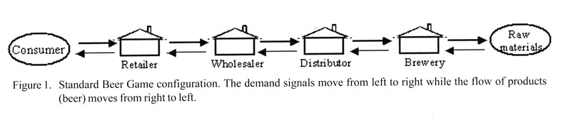
A complete description of the BG has been developed by Sterman [20] . It represents a distribution chain with four stages (positions), each managed by one or two players (Figure 1). The task of the chain is to supply consumers with beer according to demand, while minimising total system costs. Starting from the raw materials, the first position is the brewery, which produces and delivers beer to a distributor (second position). The distributor, in turn, supplies a wholesaler (third position), who supplies a retailer (fourth position). The retailer sells beer to consumers according to their demand.
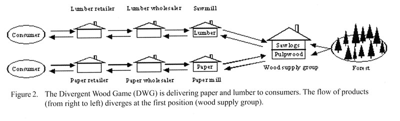
The WGs also have four stages (Figure 2), but include two chains with the forest as a common source for raw materials. At the first position (wood supply group), the flow diverges into two branches, as pulpwood and sawlogs are distributed to a paper mill and a sawmill. The two mills correspond to the distributor position in the BG (second position), and supply wholesalers and retailers with their respective products. This variant is referred to as the Divergent Wood Game (DWG) (Figure 2).
Display large image of Figure 1

Display large image of Figure 2
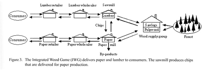
A second variant of the WG was developed to further increase relevance to forest industries. In this variant, chips are separated from lumber products at the sawmill (second position), creating an additional point of divergence for the lumber branch (Figure 3). Chips are thereafter delivered to the paper mill, and mixed with pulpwood for paper production, thus creating a point of convergence. A third point of divergence is introduced as the paper mill produces paper and by-products, where the latter is removed, and thereby not considered further in the game. This game is referred to as the Integrated Wood Game (IWG).
The proposed changes introduce parallel interactions to the systems. These are defined as interactions where a given actor may be affected by events occurring in a parallel channel in a supply network [26] .

Display large image of Figure 3
One or two individuals manage each position in the games. The game is normally played for 35 cycles (weeks), where each cycle involves receiving raw materials, production (paper mill and sawmill), order processing, shipping products, inventory control and placing new orders. Each position keeps a record of inventory development and sequence of placed orders. Prior to the game, each retailer (fourth position) is supplied with a deck of cards representing final consumer demand. All experiments with the WGs used a sequence of consumer demand identical to the BG: 4 units per week for the first four weeks, and 8 units per week for all the remaining weeks of the game. There is a four-week lead time between positions, except for the first position, (brewery and wood supply group) which faces a three-week lead time.
Inventories and goods in transit are visible to all players. Concerning information on orders, the players may only see orders from their immediate customers, and may not communicate this information to other players. Consumer demand is only viewed by retailers.
Players are not allowed to deliver more products than the sum of received orders at any time. If a player has insufficient inventory to deliver according to orders, the player is penalised with a weekly cost for each unit in the backlog of orders.
For the points of divergence and convergence, some restrictions with relevance to the forest sector apply:
Altogether, DWG has been run three times, and IWG has been run six times. The participants were 3rd and 4th year students in forestry logistics courses at the Swedish University of Agricultural Science and the Agricultural University of Norway. All games were played during 2000 - 2002.
Performance measures
The results are judged in terms of total supply chain costs, where cost minimisation is the target. Cost assumptions for the WGs are identical to the ones used in the BG. The two cost drivers are inventory, with a weekly unit cost of 0.5 US$, and backlogs of unfilled orders, with a weekly unit penalty of 1.0 US$. As the WGs consist of two branches, the average result for each position is used in comparisons with the BG.
To measure supply chain dynamics, basic statistics (mean, maximum value and standard deviation) of the sequence of orders placed by the players are used. The mean of orders indicates whether demand grows as a result of over-ordering during the playing period. The standard deviation is used to indicate changes in demand variation. As a result of flow divergence in IWG, demand for sawlogs doubles at the second position (sawmill). Consequently, orders for sawlogs in IWG (sawmill and wood supply group) are reduced by 50 % before comparing results with the BG.
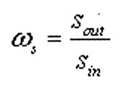
Amplification of demand variation is measured as the relative increase in standard deviation of the orders placed. This is defined as:
 (1)
(1)
where ωs is the amplification of demand variation by a given actor, sout is the sample standard deviation of placed orders by the actor, and sin is the sample standard deviation of orders received by the same actor.
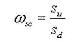
Amplification of demand variation estimated according to (1) provides a relative measure of how each position has contributed to amplifying demand variation. To represent a measure applicable to a complete supply chain (or a part of such), ωsc is used:
 (2)
(2)
where ωsc is the relative amplification of demand variation from start to end of a supply chain (or part of such), su is the standard deviation of the orders placed by the actor furthest upstream in the supply chain and sd is the standard deviation of demand (order sequence) received by the actor furthest downstream in the supply chain. Commonly, sd is the standard deviation of consumer demand.
Consequences of demand distortion
In order to study how demand distortion affects operations upstream in the supply chain, 3 IWGs are arranged such that their first positions (wood supply group) converge and order wood from the same forest. The forest resources are represented by a network of nodes located on a hexagon (forest area). Each node represents a supply point with a fixed weekly supply of wood (Figure 4). It is assumed that the mills are located on their respective peripheral segments of the hexagonal forest. In this way, higher demand requires wood from a greater number of nodes which translates into longer transport distances. For each wood supply group the forest is divided into 4 zones between which unit costs for log hauling differ. This enables studies of how amplified demand variation may influence log hauling costs.
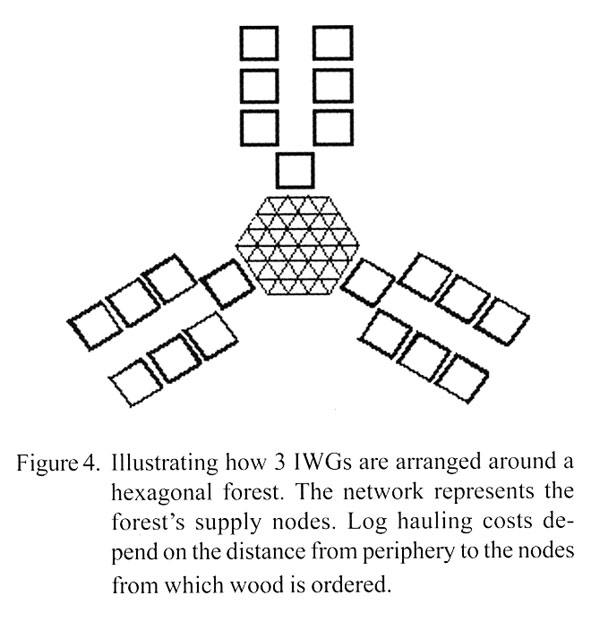
The most remote zone (zone 4) represents import with unlimited supply. Transportation costs per load are 0.5 US$ for zone 1, 0.75 US$ for zone 2, 1.0 US$ for zone 3 and 1.5 US$ for zone 4. Each chain seeks to procure wood from the nodes that minimise the chains transportation costs. For each IWG the total costs of log hauling are compared with values of ωsc (2).
RESULTS
The total supply chain costs in the BG (N=11) are on average 2,028 US$ [21] . Results from experiments with the WGs (Table 1) indicate that the average total costs are somewhat higher (2,259 US$) for the DWG (N=3) and substantially higher (3,443 US$) for the IWG (N=6). The costs for each position in the DWG are similar to costs from the BG, except for the first position (wood supply group), which has approximately twice the costs of the corresponding position in the BG (brewery). The experiments with the IWG produced considerably higher costs, particularly for the first and second positions (mills / distributor) (Table 1).
Table 1. Average costs (US$) for each positions, and average total costs of BG [21] , DWG and IWG.
| Position | BG | Costs (US$) DWG |
IWG |
| Fourth | 383 | 358 | 401 |
| Third | 635 | 512 | 691 |
| Second | 630 | 542 | 1,465 |
| First | 380 | 847 | 886 |
| Total | 2,028 | 2,259 | 3,443 |
The statistics presented in Table 2 enable a comparison of the dynamics of the different games.
The mean order appears to be similar for the fourth and third positions in all variants. The DWG has higher mean orders for the first position in particular, while the IWG appears to have higher mean orders for the first and second positions, indicating that over-ordering happens more frequently in the IWG.
Studying the figures of the maximum order placed, a similar pattern is revealed. It is particularly the first position in the DWG where the maximum order is greater than observed in BG. The IWG, however, has higher values for all four positions, the two upstream positions in particular.
The standard deviation of orders generally increases from the fourth position, close to the market, to the first position (Table 2). The standard deviations of order rates found for the positions 2-3 are somewhat higher for the DWG compared to the BG. For the first position in the DWG (wood supply group), which is the point of divergence, the standard deviation of the order sequence is 20% higher than the corresponding position in BG (Table 2). The highest standard deviation was observed for the first position in the IWG, being approximately twice the standard deviation observed for the corresponding positions in BG (Table 2). Also for the second and third position the IWG has higher standard deviations of the sequence of orders than observed in the BG.
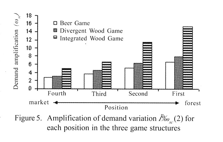
Figure 5, displaying the amplification of demand variation ωsc (2), summarises results well concerning the dynamics observed in the 3 different game structures. The demand distortion measures presented show similar rankings of the supply chain configurations. Results from the BG indicate the lowest degree of demand distortion. In these studies demand distortion in DWG was on an intermediate level, while the results from IWG indicate considerable demand distortion.

Display large image of Figure 5
Consequences of instability and complexity
For these studies, the more complex supply chain structures resulted in higher degrees of instability. System instability and amplification of demand variation has a clear effect on operations planning for upstream actors in the supply chain. Table 3 presents results from an experiment combining three IWGs in one larger system, where each chain is supplied from the same forest (Figure 4). Results show that the chain with the lowest values of ωsc also was able to procure logs closer to the chain, resulting in lower unit costs of transportation.
Table 2. Summary of average order statistics for Beer Game (BG), Divergent Wood Game (DWG) and Integrated Wood Game (IWG).
| Mean order | Max order | Standard deviation of orders | |||||||
| Position | BG [2] | DWG | IWG | BG [21] | DWG | IWG | BG [21] | DWG | IWG |
| Demand | 7.5 | 7.5 | 7.5 | 8 | 8 | 8 | 1.3 | 1.3 | 1.3 |
| Fourth | 7.4 | 8.1 | 8.8 | 15 | 17 | 30 | 3.6 | 3.8 | 3.9 |
| Third | 8.6 | 8.1 | 9.8 | 19 | 26 | 32 | 4.8 | 5.8 | 7.5 |
| Second | 9.1 | 8.5 | 13.2 | 27 | 30 | 49 | 6.7 | 8.2 | 11.6 |
| First | 9.0 | 9.3 | 13.9 | 32 | 60 | 74 | 8.5 | 14.6 | 17.2 |
Table 3. Unit costs of log hauling (US$/load) and relative amplification of demand variation (ωsc) for 3 IWGs.
| Chain A | Chain B | Chain C | |
| Unit cost (US$/load) | 1.19 | 1.12 | 1.05 |
| ωsc | 20.13 | 19.34 | 12.53 |
DISCUSSION
As supply chain complexity increases so does the degree of demand distortion (Table 2, Figure 5). The same basic mechanisms which result in demand distortion can be observed in all the game configurations, however, the outcomes of order decisions vary between supply chain configurations. To clarify this, we start the discussion with describing a cycle of 5 events and control systems, proposed by Houlihan [11] , in which interactions between customers and suppliers leads to distorted demand signals. We then describe the role of demand distortion in the BG and WGs along with some advice concerning how to measure demand variation. Possible effects of distorted demand on upstream operations as well as relevance of assumptions and configurations in relation to the prevailing conditions in the forest industries are also discussed. We end the discussion by presenting arguments that show the relevance of presented results, and suggest how to prevent demand distortion from negatively affecting performance in the future development of forest industry supply chains.
Demand distortion mechanisms
In the context of the forest products industry Hameri [7] describes how industrial dynamics develops between customer and supplier according to the mentioned cycle of 5 events. For a papermill and its wholesaler, the cycle may start with an upswing in customer requirements (increased orders), leading to increased requirements for mill capacity and/or materials (event 1). If the mill cannot deliver within the expected lead time, it leads to the customer getting an impression of shortages of capacity and/or materials (event 2). The common reaction to perceived shortages is customer over-ordering (event 3). The over-ordering, in turn, results in unreliable delivery from the mill (event 4). Finally, perception of increased uncertainty motivates the customer to increase the volume of safety stocks, which require additional orders to reach the new target inventory (event 5). The customer over-ordering (event 3) and increase in safety stocks (event 5) give the mill the (distorted) impression of increased consumer demand, thereby completing the cycle. A similar cycle of events is often described as the "the evil circle" by BG and WG participants. There is, however, little consistency concerning where in the chain demand distortion is greatest, illustrating the system instability.
Measuring demand distortion
Over time, the quantity ordered and the quantity delivered will coincide. Hence, it is only during shorter time periods, when companies act on distorted demand information, or when pursuing strategies involving changes in inventory levels that the quantity of orders sent to vendors differs from the quantity of orders received from customers. Thus, demand distortion in supply chains studied over extended periods of time can be reduced to amplification of demand variation, quantified by ωs (1) for the contribution of a single actor and ωsc (2) for the combined contribution of the supply chain, or part of such.
Amplification of demand variation is most prevalent in IWG (Figure 5, Table 2). As can be seen in Table 2, over-ordering contributes considerably to demand distortion, since the mean of orders placed are considerably higher than consumer demand. Considering that the playing period is 35 weeks (2/3 of a year), this demonstrates the importance of monitoring the mean order level as well as ωs, in order to detect and remedy over-ordering in the system. When using methods to quantify demand distortion that adjust for differences in flow volumes, such as measurements based on the coefficient of variation [5] (the ratio of standard deviation to the mean), these effects are not discovered. If the causes of a particular problem are not properly revealed, effective measures to remedy the problem will be hard to discover and implement. Adjusting for differences in product flows is appropriate when access to relevant data is prevented, for example when production represents divergent flows with variable and uncertain product outcomes.
Corrections to steady state
The cycle of events leading to demand distortion is symptomatic for any system dominated by stock control ordering. In the framework proposed by Fowler [4] , stock control ordering systems, such as Just-In-Time and Kanban are actually adaptations of generic feedback control where system instability can arise as a combined result of time lags and controller gain (reaction to discrepancies in target stock). Longer time lags between changes in system state and corrective measures result in lower success in correcting the situation. Long time lags combined with a high controller gain, to quickly regain control of the system, result in considerable system instability [4] . A series of cascading feedback loops, such as found in the BG, makes correction to steady state increasingly difficult. For these reasons complex systems should also include a feed-forward control loop aimed at predicting the effects of major changes in system environment, while the multitude of minor disturbances are trimmed with the use of low controller gain feed-back loops [4] . Furthermore, the stability of complex systems can be considerably improved through efforts in lead time reduction [22] .
Demand distortion in BG and WG
In order to better understand the specific order behaviour of an actual stock manager within a system, the cycle of 5 events should be viewed in the framework of a generic stock management system [21] . The generic stock order decision rule is based on only locally available information and recognizes three motives for ordering at any given point in time [21] . These include:
The emphasis put on each of these motives depends on the expected acquisition time lag to receive the ordered quantities. The expected acquisition time lag is short when the supplier has excessive inventory, and increases in cases where suppliers' inventory is small or depleted.
Quantification of player reactions in relation to the terms of the generic stock decision model is based on the degree to which the players emphasise adjustments in stock or supply line in their order decisions. Sterman [21] defines αS as the fraction of the stock discrepancy ordered each period, and αSL as the fraction of the supply line (materials on order) discrepancy ordered each period. Initial instability in the BG is commonly associated with students mainly considering their inventory/backlog when making ordering decisions (high αS), failing to take into account quantities on order (low αSL). This result is not surprising since the supply line, contrary to the inventory, is never recorded by the players, and since the time delays make it difficult for the players to keep track of quantities on order.
Although the basic mechanisms resulting in demand distortion are the same in each configuration, effects are different, resulting from the increased complexity with multiple interdependencies between positions. It is acknowledged that other mechanisms for demand distortion exist, as proposed by Lee et al. [15] . These, however, are based on changing product prices, existence of several sources of supply or existence of competitors, and are for these reasons outside the scope of this paper.
In the WGs the relative content of sawlogs and pulpwood in the product mix delivered from the forest is restricted, making the degree of demand distortion dependent on the degree to which the development of demand signals in the two branches is synchronised. Consider a situation where demand in the paper branch increases faster than demand in the lumber branch. Hence, the papermill enters the cycle of perceived shortages (event 2), over-ordering (event 3) and attempts to increase stocks (event 4) earlier than the sawmill. The wood supply group then gets the impression of rapid increase in consumer demand for paper compared to that of lumber. This induces a forced over-ordering of sawlogs by the wood supply group, observable in the games through high values of ωsc, and increased mean of orders. More profound effects (forced over-ordering of sawlogs) are observed in cases with rigid restrictions concerning the relative content of sawlogs and pulpwood in the product mix.
In the IWG parallel interactions [26] are introduced between branches through the supply of chips from the sawmill to the papermill. The relative content of chips and pulpwood allowed in paper production, determines the degree to which the papermill may compensate for perceived pulpwood shortages by increasing chips orders, or the other way around. The convergent restriction can therefore generate perceptions of both pulpwood and chips shortages (event 2). In the case of chips shortages, the ability of the sawmill to meet these is constrained by the fixed fraction of the sawlogs that is converted to chips. Hence, shortages in raw materials for the paper mill can also generate over-ordering (event 3) in the lumber branch. The sawmill must continuously consider the trade-off between inventory of one product and backlog of the other, particularly in cases where demand distortion develops differently in the two branches. In situations where the sawmills' chips inventory is depleted, the acquisition time lag for chips to the paper mill increases and exceeds that of pulpwood.
The situations in DWG and IWG both require stock order decisions rules with a high emphasis on the supply line (high αSL compared to αS) in order to keep demand distortions at acceptable levels.
Consequences of demand distortion for wood supply operations
The strongest effects of demand distortion are experienced by companies far upstream in supply chains [3] . Furthermore, as long as control systems allow, demand variation will amplify [23] . This makes forest operations and forest products industries potentially exposed to demand distortion.
Table 4 shows that chains with highly distorted demand signals (high ωsc) were forced to procure wood further from own location resulting in a higher unit cost of transportation. Haartveit and Fjeld [6] showed that the rate at which transport distances increase when mill requirements increase, varies widely for different wood procurement areas, depending on the spatial distribution of forest resources and the spatial extension and quality of the road network. An equal increase in wood demand would result in some wood procurement areas facing an increase in transport distances that was 20-40% higher compared to the most favourable wood procurement areas [6] . Hence, effects of demand distortion on the forest industry, forest operations included, will likely show spatial variation.
Relevance of assumptions and constraints
The wood games are used to simulate the challenges, which will be met when introducing a greater degree of customer orientation in the forest sector.
From a perspective of systems stability, the realism of the games' configurations should be examined. Relevant aspects of the configurations include: time lags, controller gain, restrictions on divergence as well as the degree of parallel interactions and restrictions on information flow.
Average times for wood procurement from stump to mill for large-scale forest operations often exceed three weeks. The time required for communicating revision of delivery plans varies considerably, depending on the organization, however, a monthly revision cycle is typical, resulting in a total wood supply lead time of at least 6 weeks. Average lead times for delivery from paper mills used in a study by Hameri and Nikkola [8] varied between 3 and 8 weeks. In the WGs the lead time for wood supply is four weeks (assuming that the ordered quantity is in stock). Thus, the primary lead times are shorter in the WGs than would be realistic for the forest sector.
Applying the common strategy of maximised production with high and even capacity utilisation, volume flexibility in large papermills is inherently low and controller gain is limited [16] . Concerning forest operations, however, Helstad et al. [10] report values of volume flexibility as high as 30%. The DWG and IWG, however, have no restrictions concerning the volume flexibility in forest operations, making the potential controller gain of the games greater than reported values for forest operations. The WSs are not hampered by seasonal supply variability, which typically results from climatic factors.
In wood procurement, product mix flexibility (percentage of sawlogs or pulpwood) may be changed by up to 30-40% for a monthly period [9] . Assuming 40% pulpwood in the total delivery as normal, this indicates that the percentage of pulpwood delivered from the forest could be varied between 26% and 54% on a monthly level. In IWG the percentage of pulpwood in deliveries from the forest must be between 30% and 40%, corresponding to a product-mix flexibility of 14% for pulpwood and 8% for sawlogs, which seems stricter than can be obtained through careful planning of forest operations.
The low product diversity, with two products at each mill) in the WGs constitutes a major simplification of the system. In contrast, a larger sawmill produces up to 1000 different product variants. Still, in order to learn from studies of complex systems, complexity in these models must be kept at controllable levels.
The greatest differences between WGs and reality are the absence of pricing strategies, the absence of competitors and alternative sources of supply. Requiring that all trade be done within each supply chain increases degrees of parallel interactions in the system. At first glance such isolated studies of supply chains may seem irrelevant. On the contrary, it is argued here that this situation is highly relevant when seeking to identify possible consequences of introducing a greater degree of customer orientation in the forest sector. This translates to a situation where inventories are reduced [1 , 12] , companies are more closely integrated [1] , for example through partnerships [7] , and single sourcing strategies [13] , and competition extends to being between supply chains rather than between isolated companies, a well known development seen in other industries. In all, this leads to increasing the proportion of the trade occurring within supply chains, compared to between supply chains.
Concerning access to information in the supply chain, all inventory and goods in transit are visible at all times to all actors, and the only confidential information is order levels. Thus, the player's access to information exceeds what is normally available in real supply chains. Considering the abundance of information, and the simplicity of the environment in the WGs, the amplification of demand variation is impressive. Knowledge of inventory levels is apparently not sufficient for successful management of supply chains. Increasing customer orientation while reducing inventories in forest industry supply chains requires increased transparency of information between the actors. Even within vertically integrated companies, demand is commonly distorted because these companies frequently consist of autonomous organisational units with limited transparency of demand and inventory information [11] .
Without increased information transfer, inventory reduction often leads to instability [26] . In the forest industries, however, the relationships between customers and suppliers are commonly described as adversarial [25] . Oftentimes transparency of inventory and sales information are avoided, and selling and buying take place according to most profitable bid at the time of sales. The few existing publications on customised production in the forest industries emphasise few, loyal customers where the traded volume and the degree of trust are high [13 , 14] . The increased degree of information transfer required when increasing customer orientation becomes an emerging challenge for actors that consider pursuit of this strategy. Complex information flows with high frequencies of transactions put limitations to the number of customers that can be served using this strategy. Additionally, the nature of manufacturing in divergent flows, where the volume and quality of each product are subject to variation, suggests that there will always be a percentage of the total production that is produced in anticipation of future demand.
CONCLUSIONS
Use of the WGs as a simulation tool provides us with insights about some of the challenges associated with increasing customer orientation in supply chains in the forest sector. While demand distortion has been shown to exist close to the markets in the supply chain, this effect has, until recently, been negligible upstream in the chain. This is because of the typically prognosis-based management of wood supply.
This framework of analysis may be used to simulate the effects of increasing customer orientation, inventory policies, and interdependencies in different supply chain configurations at the same time as including the human elements of customer decision-making.
The increase of costs and demand distortion observed for complex supply chain configurations are important to consider as interdependencies increases between customers and suppliers in the forest sector.
Obviously, the degree of divergence is in reality much greater than shown in these examples, as is then the difficulty of achieving high service levels and low inventories while aiming to increase the degree of pull based flows in the supply chains.
The further development of decision support solutions should therefore not ignore basic functionality such as providing transparent information on demand and inventory to actors in supply chains, thereby enabling them to respond rapidly and correctly based on undistorted information on demand. This point is essential when pursuing intuitively contradicting targets such as high capacity utilisation, reduced lead times, reduced costs, and increased service levels.
AUTHOR CONTACT
Mr. Haartveit can be contacted by e-mail at -- erlend.haartveit@skogforsk.no
REFERENCES
[1] Carlsson, D. and M. Rönnquist. 1999. Wood flow problems in Swedish forestry. Skogforsk Report No. 1, 1999. Uppsala, Sweden. 48pp.
[2] Fjeld, D. E. 2001. The Wood Supply Game as an educational application for simulating industrial dynamics in the forest sector. In: Sjöström, K. and L-O. Rask, [Eds]. 2001. Supply Chain Management for Paper and Timber Industries. Timber Logistics Club. pp:241-252.
[3] Forrester, J. W. 1958. Industrial dynamics - a major breaktrhough for decision makers. Harward Business Review, July-August, 1958.
[4] Fowler, A. 1999. Feed-back and feed-forward as systematic frameworks for operations control. International Journal of Operations & Production Management, Vol. 19(2):182-204.
[5] Fransoo, J. G. and M. J. F. Wouters. 2000. Measuring the bullwhip effect in the supply chain. Supply Chain Management, Vol. 5 (2):78-89.
[6] Haartveit, E. Y. and D. E. Fjeld. 2000. Interregional variations in transport net geometry - an analysis of wood procurement areas for Norwegian sawmills. In: Sjöström, K. [Ed.]. 1999. Logistics in the Forest Sector. Timber Logistics Club. pp:165-187.
[7] Hameri, A-P. 1996. A method to avoid demand amplification in bulk paper distribution. Paperi ja Puu - Paper and timber, Vol. 78(3):102-106.
[8] Hameri, A-P. and J. Nikkola. 1999. Demand amplification in supply chains of mills close to and far from main markets. Paperi ja Puu - Paper and Timber, Vol. 81(6):434-438.
[9] Helstad, K. 2000. Skiftformer för framtidens råvaruförsörjning - flexibilitet, kostnader och arbetsmiljö. [Shift forms for raw material supply in the future - flexibility, costs and working environment]. MSc. Thesis, Swedish University of Agricultural Sciences, Div. of Forest Technology, Umeå.
[10] Helstad, K., A. E. Nilsson, and D. E. Fjeld 2001. Volume flexibility in wood procurement - costs and constraints for adjusting supply chain strategy. In: Sjöström, K. and L-O. Rask, [Eds.]. 2001. Supply Chain Management for Paper and Timber Industries. Timber Logistics Club. pp:143-162.
[11] Houlihan, J. B. 1985. International Supply Chain Management. International Journal of Physical Distribution and Materials Management, Vol. 15(1):22-37.
[12] Högnäs, T. 2000. Towards Supplier Partnerships in Timber Harvesting and Transportation. Forestry Publications of Metsähallitus 37.
[13] Peterson, J., S. Peters, E. Wachtman and S. Johnson. 1999. Customer Intimacy Drives Success at Boise Cascade Corporation's Western Oregon Lumber - Shifting focus from production to customers' needs. Target - The Journal of the Association of Manufacturing Excellence Vol. 15(3):26-31.
[14] Kozak, R. A. and D. H. Cohen. 1997. Distributor - Supplier Partnering Relationships: A Case in Trust. Journal of Business Research, Vol. 39:33-38.
[15] Lee, H. L., V. Padmanabhan and S. Whang. 1997. Information Distortion in a Supply Chain: The Bullwhip Effect. Management Science, Vol. 43(4): 546-558.
[16] Lehtonen, J-M. 1999. Supply chain development in process industry. Acta Polytechnica Scandinavica IM No. 4.
[17] Macbeth, D. K. and N. Ferguson. 1994. Partnership Sourcing - An Integrated Supply Chain Management Approach. Pitman Publishing, London, UK.
[18] Metters, R. 1997. Quantifying the bullwhip effect in supply chains. Journal of Operations Management, Vol. 15:89-100.
[19] Mosekilde, E. and E. R. Larsen. 1988. Deterministic Chaos in the beer production-distribution model. System Dynamics Review, Vol. 4 (1-2):131-147.
[20] Sterman, J. D. 1984. Instructions for running the Beer Distribution Game D-3679, Systems Dynamics Group, MIT, E60-383, Cambridge, MA 02139.
[21] Sterman, J. D. 1988. Deterministic chaos in models of human behaviour: methodological issues and experimental results. System Dynamics Review, Vol. 4(1-2):148-178.
[22] Towill, D. R. 1996. Time compression and supply chain management - a guided tour. Supply Chain Management, Vol. 1 (1):15-27.
[23] Towill, D. R. and del Vecchio, A. 1994. The application of filter theory to the study of supply chain dynamics. Production Planning and Control, Vol. 5 (1):82-96.
[24] van Ackere, A., E. R. Larsen and J. D. W. Morecroft 1993. Systems thinking and business process redesign: an application to the beer game. European Management Journal, Vol. 11 (4):412-423.
[25] Vlosky, R. P., E. J. Wilson, D. H. Cohen, F. Fontenot, W. J. Johnston, R. A. Kozak, D. Lawson, J. E. Lewin, D. A. Paun, E. S. Ross, J. T. Simpson, P. M. Smith, T. Smith and B. M. Wren. 1998. Partnerships versus typical relationships between wood products distributors and their manufacturer suppliers. Forest Products Journal. Vol. 48(3):27-35.
[26] Wilding, R. 1998. The supply chain complexity triangle - Uncertainty generation in the supply chain. International Journal of Physical Distribution & Logistics Management, Vol. 28(8):599-616.