July, 1998, vol.9 no.2
T.S. Palander
University of Joensuu
Joensuu, Finland
The author is a Researcher at the University of Joensuu, Department of Forestry.
ABSTRACT
Timber procurement is part of the flow of wood from forest to production. In the present study, it is referred to as timber flow, which consists of logging, roadside inventory, transportation, and mill inventory functions. Local timber flows should be managed by tactical means of decentralized decision making (DDM), which are facilitated by dynamic models of a decision system. The technique consists of several hierarchical negotiation levels which can solve a local procurement problem by the technique of functionally decentralized decision making (FDDM). Models describing the system are also bigger and more complicated than models which are constructed for geographically decentralized decision making (GDDM). Consequently, the models may cause different dynamic results. Therefore, this study has two main objectives: 1) to introduce a technique of GDDM and 2) to consider the effects of the time-factor using dynamically determined functions of local procurement. Using this application, the system can be controlled for balancing timber flows, because the system's internal adjustment process is defined with higher precision; the extra costs caused by a disturbance can be diminished by adjusting the durations of local timber-flow functions. The implications of these results for improving decision making (DM) of local timber procurement in Finland are discussed.
Keywords:Buffer stock, cumulative cost curve, dynamic linear programming (DLP), tactical.
INTRODUCTION
During the last three decades, the issue of decision making (DM) of the wood procurement schedule has been addressed through various forms of mathematical programming, such as dynamic programming, linear, quadratic, and separable programming; non-linear programming or gradient methods; and simulation. In studies conducted abroad, these operation methods have been applied for harvesting and transportation with cost optimization [1, 5, 6, 7, 10, 11, 20, 21, 22].
In the Finnish forest industry, the variations of linear programming (LP) have usually been used for a similar optimization context. Therefore, many applications of this method have been proposed [8, 16, 17, 23, 31]. According to these studies, general linear optimization with constant and static parameters has been the method preferred most often, especially within long-term (one year) planning problems at the highest echelons of timber procurement divisions. The time scale of the plan has not yet been considered within the local tactical DM context. That tactical decision should be based on a short-term plan, e.g., for two months, which is adjusted for fast changes in circumstances (disturbances) in the problem context.
Often a short-term model has been used for solving problems in which transportation has played a central role. Therefore, the models have been designed for partial stage management of timber flows overlooking an option of integration to manage the entire logistics timber flows from the stump to industrial products [23]. Industrial standards for mills' timber demands have become more demanding during the past few years. On the other hand, high real interest rates for short-term investments and financial purposes have influenced the total costs of timber procurement. Furthermore, many other time related factors have also stimulated progressively growing interest in reducing the logistics costs to manage the entire timber flow efficiently.
As a response to these criteria changes, the Finnish forest industry has increased the control (operational modelling) over timber flow in the direction of having less in-system inventory on hand. This is known as just-in-time (JIT) inventory [3, 13]. Because of JIT, criteria of the local tactical DM have also changed. Besides cost minimization, buffer stocks of timber flow should be decided by local decision makers, because changes in their timber order can happen every day. The changes cause additional costs if buffers do not include enough timber to satisfy timber order. Therefore, multiple objectives should be handled by a DM method which comprises a system with local tactical models.
To support timber procurement management, various methods or techniques can also be used in DM. According to Keipi [17], the development of techniques used in the DM of wood procurement in Finnish forest industry companies may be divided into five phases:
The DDM of timber procurement means that most often decisions are left to the lower hierarchical levels of an organisation [17]. Furthermore, two levels can be easily included in DM systems to support the work of a decision-making group (DMG). Accordingly, the DM of a small DMG has been more relevant for local DM than for individual or hierarchical DM.
On the local level, it could be argued that the great changes in short-term DM have caused problems in the DMG's DM. To solve these problems, the head of wood procurement divisions has paid special attention to locally integrated operational and tactical management. So far, however, tactical management has not been used properly. First, tactical planning should include an optimization of activities of the business (utilization rates, productivity, and contracts), in which the solution should be a new partial adaptation for a utilization rate of capacity, while the overall capacity is not changed [27]. In this context, the business is the timber procurement from stump to mill; the capacity is determined by the higher hierarchical level as the existing timber procurement plan and the budget; the contracts are defined as the market stands and the machines (productivity) owned by private contractors; and the partial adaptation or adjustment means that DMG designs the new short-term plan.
Secondly, in Finland since the late 1960s there has been a long tradition of FDDM, which has greatly affected decision makers' thinking and the existing tactical applications. The Finnish literature on organisations has paid much less attention to geographical decentralizing, although GDDM techniques should be applied at the local level.
Thirdly, in generation of tactical decision alternatives for small geographical units, dynamic DM systems would be more practicable than static systems. If the problem of cost minimization is solved using a static system, the solutions represent a single moment in time. DMs are assumed to be capable to adapt their decisions to disturbances (external shocks) by instantaneously controlling the system without adjustment costs. This has been usual when optimizing models of wood procurement are used in capital management of monetary flow. Thus, companies' static models have been long-term models. Consequently, the elements of the system, including capital, have been assumed to be variables. To avoid these problems in the dynamic inconsistency [4], tactical DM should be provided with a dynamic system. This kind of system is also better to characterize as the time variant system [28].
If dynamic systems would be used for generation of tactical short-term schedules, total costs of timber flows could be increased by an adjustment cost of the capital based on time-related inputs, such as changes of timber order, timber inventory resources, and limits of budget. In this study, they are referred to as the time-factor. Under these local conditions, the capital is used as an explicit (fixed) cost-factor. This will cause internal adjustment costs in the system, when buffer stocks are used as the adapter.
The research problem is to introduce a useful tactical implementation for the GDDM, and to test the implementation with the illustrative experiment based on empirical data. At the system level, the contribution of this study is to develop the preliminary dynamic application to a tactical decision process of the independent and local profit units. The DLP-model is applied, in which time-varying parameters are used in the models' weight parameters and time-related parameters are used in the models' constraints. The hypothesis has three parts: the time factor influences local total and unit costs and the tactical decisions of local management operate with time, thus dynamic tactical applications are useful in the GDDM.
GDDM TECHNIQUE
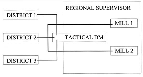
General information connections of a region of the experiment are described in Figure 1. For geographical decentralizing, a region was divided into smaller distinct districts operating as the local echelon in the divisional hierarchy and managing their purchasing, logging, and transportation operations independently. In functional decentralizing, the responsibilities of these operations were separated based on the hierarchy, functions, and the meaning of the decision (operational, tactical). Accordingly, the DDM was also divided into two distinct techniques, which were based on those different principles used in delegating responsibilities within a decentralized organization:
Figure 1. Crosses of lines depict a region's information connections in a decentralized organization. Districts are independent profit units.
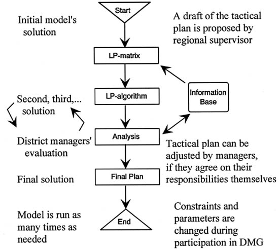
Figure 2. General principles of the GDDM.
The GDDM was a usual negotiation and optimization process, which provided the consensus decision for the DMG. This procedure is consistent with the steps of the methodology recommended by Hotvedt et al. [14] except that they used the principles of the FDDM. General principles of the GDDM are described in (Figure 2). For reaching the consensus as to the best compromise schedule, the regional supervisor controlled and coordinated the districts' operations via participative management. In the first phase, the district managers updated the common information base and the supervisor prepared drafts for the districts according to the method of Field et al. [9]. According to that method, the solution values for each district were then used in the model of the initial plan which was based on the local information. In the second phase, the managers had the option of negotiating the final plan (a tactical plan) together.
Before the models could be formulated, prior defining of local goals for the DMG's tactical planning was necessary. A pattern of these goals was also used as criteria of the DMG for the consensus decision about the timber procurement schedule. To find out initial directions for DM, the use of the minimum of the discounted total costs and the maximum of the timber delivery was obvious (identified by the company). According to interviews by Keipi [17], managers of a functionally decentralized organization also had specific criteria for the FDDM. Here, the local criteria (local goals) were based on those of functional managers, but the new synthesis was defined for the GDDM purposes. Consequently, the local criteria of the district managers were as follows:
The first and the most important criterion from these were to satisfy mills' qualitative and quantitative timber demand when the members of the DMG indicated their preferences. In this context, more attention was paid to the quantitative demands. These demands were equally divided among the distinct districts according to the region's timber orders. The qualitative requirements could be defined about different tree species and requirements for the timber material, but these were outside the scope of this study. The idea was to come up with the time-oriented criteria relevant for tactical DM when dealing with local conditions. The order of importance of the other criteria was not ranked.
Coordination of the initial plan into one tactical plan was made using the methology of parametric programming of the RHS for multi-objective analysis. For the GDDM the model was the pure local model with local cost weights and buffer parameters, which completely integrated the district's timber procurement functions. Therefore, the model's small changes to meet the practical management needs were agreements done by the participation of the district managers. In conventional FDDM models integration was made by using aggregate input and output data of the higher hierarchical level. The final model was the solution of the final reformulation of the evaluated model solved after the preceding negotiation. Thus, the tactical decision was the result of the "planning cycles", where negotiations of the DMG and predestined number of model runs were made with the cooperation of the regional supervisor.
DYNAMIC TACTICAL APPLICATION
Keipi [17] applied a DLP model in the FDDM at the highest echelon of a division, referred to in this study as the conventional model. To extend his findings, this study was concerned with the use of local DLP models in the GDDM at the local level of the division. In particular, the tactical optimizing models [25] were applied for the experiment of the GDDM. For more about the tactical formulation of DLP and its applications see Palander [25]. All models could be solved by the Simplex algorithm and the experiment was played by undergraduates of the university of Joensuu.
The application comprised the dynamic DM system that investigated the problem as a logging and transportation system (Figure 3). The basic input data of the system have been introduced in two studies [24], [25]. Besides the decision criteria, the decision variables, states, and relationships of the system dynamics were described, computed, and controlled by ordinary ways using the DLP models' parameters and constraints. Therefore, the DLP results provided a good form of the parametric solution for the time-related sensitivity analysis, and for considerations of the application for the GDDM.
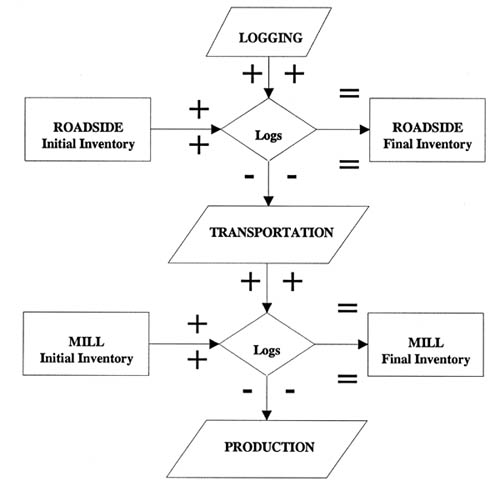
Figure 3. Monetary and material flows were optimized using the program that included the functions of logging, transportation, and inventorying, both at the roadside and at the mill.
In the experiment of the tactical application of the GDDM, a new timber procurement schedule had to be prepared for a problem that occurred when the region's timber order changed while the mills' timber demands had not changed. Following the GDDM, the district managers responded to the new situation and tried to adapt their decisions with the cooperation of other districts, but the managers could not cope with the situation using the initial model of the FDDM. The solution of this initial model is provided in Table 1 and Figure 5. Therefore, assembling the DMG was necessary and the managers reformulated the entire initial model, applying the local duration of timber flow functions using the buffer stocks of the roadside inventories of timber flows.
The GDDM continues by the demonstration of a simple changing process from the initial model to the final model. Before the cycles (reformulation) started, the initial solution was presented to the districts' managers. They individually evaluated the solution in the beginning of the first cycle, but the new initial solution did not satisfy the DMG. Therefore, the DMG decided to use the logging and transportation capacities to the full, i.e., the local tactical criterion of at least 15000 m3 was transported from the districts to the mills during every decision period. This caused changes in allocations corresponding to bigger periodic logging volumes of at least 20,000 m3, 17,000 m3, 10,000 m3, 10,000 m3.
The final model coped with that tactical decision criterion, but DMG must compromise. That model was the result of two cycles of the GDDM. First, the initial model was modified by the DMG to comply with their pattern of the local goals. Unfortunately, no feasible solution was provided by this new model. Next, in the second cycle, the DMG decided to change the criterion of the buffer stocks of the standing inventories from 20 weeks to 12 weeks. This tactical change produced the final model (Model 1) used in the analyses of the hypothesis.
minimize Z1 = [
transportation
logging operations
roadside inventory
mill inventory
minimize Z2 = [
stand inventory
maximize Z3 = [
transportation
subjected for following restrictions
Region's timber order
Yikjt + Mikt-1 = Dikt, " i,j,k,t
balancing material flow;
roadside
Xijt-1 - Yikjt + Lijt = Xijt
mill inventory
Yijkt + Mijt-1 - Dikt + Mikt
initial roundwood inventories;
Xij0 = XI ij
Mik0 = MIik
timber allocation possibilities;
Mikt Mmaxikt
Mikt Mminikt
Lij Lmaxij
Lij Lminij
Yij Ymaxij
Yij Yminij
buffer stock requirements;
Lij4 LBij
Yij4 XBij
Mik4 MBik
non-negativity;
Lijt, Xijt, Yijkt, Mik 0
where
Z1 = optimum total costs (FIM),
Z2 = optimum stand inventory (m3),
Z3 = optimum transportation (m3),
Dikt = volume (m3) of timber grade i required by mill k during period t,
Lijt = volume (m3) of timber grade i logged and hauled in area j during period t,
Mikt = volume (m3) of timber grade i retained in mill inventory k during period t,
Xijt = volume (m3) of timber grade i required in roadside inventory of area j during per- iod t,
Yijkt= volume (m3) of timber grade i transported from area j to mill k during period t,
Lmaxij = maximum volume (m3) of timber grade i logged in area j during the planning hori- zon,
Lminij = minimum volume (m3) of timber grade i logged in area j during the planning hori- zon,
Mminikt = minimum volume (m3) of timber grade i required at the mill inventory k during period t,
Mmaxikt = maximum volume (m3) of timber grade i stored at the mill inventory k during per- iod t,
Ymaxijt = maximum volume (m3) of timber grade i transported from area j during period t,
Yminijt= minimum volume (m3) of timber grade i transported from area j during period t,
clijt = pre-roadside timber procurement cost per unit volume (FIM/m3) of timber grade i transported from area j,
cmik = mill inventory cost per unit volume (FIM/ m3) of timber grade i in mill inventory k,
cyijkt = transportation cost per unit volume (FIM/ m3) of timber grade i from area j to mill k at stage t,
coffit = moisture coefficient of timber grade i at stage t,
Liij = stand volume (m3) of grade i stored in area j at the beginning of the planning horizon,
MIik = volume (m3) of grade i stored in mill k at the beginning of the planning horizon,
XIij = volume (m3) of grade i stored at roadside in area j at the beginning of the planning horizon,
Lbik = volume (m3) of grade i required in log- ging in area j at the end of the planning horizon,
MBik = volume (m3) of grade i required in mill inventory k at the end of the planning horizon,
XBij = volume (m3) of grade i required at road side in area j at the end of the planning horizon,
P = annual interest rate,
T = number of discrete periods (two weeks) of the planning horizon,
K = number of mill inventories,
J = number of management areas, and
I = number of timber grades.
Among the local manager's goals, the volumes of the various stand inventories (buffer stocks) were subjected to the restrictions; the discounted total costs had to be minimized by keeping the volumes of inventories small and by satisfying the requirements of the current and future states of the timber-flow functions. Further, purchase was assumed to be included in the initial stand inventory. The parametric optimizing technique provided the structure for the construction of the constraints by which that subjection could be controlled.
Most often tactical decisions are based on time-related schedules. Therefore, the time factor is an important aspect of the GDDM. The effects of the time factor were divided into partial sub-factors (capital, interest, logging costs, and transportation costs), described as functions of time. The first was controlled by RHS parameters and latter three by weights of decision variables. Buffer stocks as a parameter could be used for combining several criteria which depended on the time. Therefore, the buffer stock was the most important criterion for the modelling purposes. Here, time was pictured as a 'coordinator' for adjustment costs of the system. Thus, the dynamic problem of the monetary flow involved with the essential capital requirements was transformed to volumes of timber flow by the buffer stock requirements of the timber-flow inventories. Capital was determined as funds accumulated in the various inventories of timber flows instead of funds accumulated in the volumes of timber delivered to the mills.
In the models, over the two months' DM horizon, the change of the capital accumulation of timber flows varied depending on allocations made during the preceding two weeks' period. This started from the first period while the buffer stocks for the final period were determined as fixed by some volumes of timber. Because of this, the states of the system could be eventually determined as the process of partial adjustment of the capacity instead of the capital. Further, in the GDDM the durations of timber-flow functions were interpreted as weeks of the local buffer stocks, which were transformed to the capital accumulation for the districts. Therefore, the state of the system was not as much stable when the solution was solved by the GDDM, and this distinguished it from the combination of the FDDM.
Buffer stocks were the manager's means to control the system. The information base included input data about the monetary and timber flows. Monetary flow was conventional to manage using budget, because its role has increased in all organizational levels. Actually, because of the local level, the budget was related to the cash flow of the funds. Timber flow was managed by the stages of the defined time accumulation. Hence, durations of timber-flow functions were important. They were used in the cumulative curve, which was presented in the figure for the stumpage sales of wood procured for the Finnish forest industry [19] .
The entire buffer time needed for securing a continuous flow of timber was about ten months: twenty weeks for stand inventorying, four weeks for logging, nine weeks for roadside inventorying, one week for transportation, and four weeks for mill inventorying. Stand inventorying as the timber-flow function was the DM criterion. The transportation function was omitted from the transformation between cash flow and timber flow. The other three partial timber-flow functions were considered separately and they were determined using the following equations:
LBij = lcoffij * (D / WEEKS) * (LIN
XBij = lcoffij * (D / WEEKS) * (X
MBik = mcoffik * (D / WEEKS) *
where
LBij= volume (m3) of grade i required for stumpage inventory in area j at the end of the planning horizon,
XBij= volume (m3) of grade i required at the roadside in area j at the end of the planning horizon,
MBik = volume (m3) of grade i required in mill inventory k at the end of the plan- ning horizon,
LINV = total logging inventory,
XINV = total roadside inventory,
MINV = total mill inventory,
LINVij = volume (m3) of grade i available in the stumpage inventory in area j at the beginning of the planning horizon,
XINVij= volume (m3) of grade i available at the roadside in area j at the beginning of the planning horizon,
MINVik= volume (m3) of grade i available in mill inventory k at the end of the plan- ning horizon,
D = region's timber order,
WEEKS = weekly length of the planning horizon,
lcoffij = buffer stock coefficient as weeks for logging inventories,
xcoffij = buffer stock coefficient as weeks for roadside inventories, and
mcoffik = buffer stock coefficient as weeks for mill inventories.
Fixed useable working was determined by means of these equations as the minimum level combined with fixed timber inventory resources; in this application it was the minimum volume requirement. This was relevant to assume for two reasons; first, the budgeting traditions of the forest industry supported it, and second, during the short-term DM horizon the decision system was subjected to the assumption of partial adjustment. Accordingly, the adjustment costs of a fixed capital are part of discounted total costs to be taken into account when conducting GDDM.
The adjustment costs were imagined as either external or internal costs. External costs can be illustrated by assuming that the capital accumulation in inventories was financed by a loan. Then the interest rate of the loan was a cost factor in cash flow determined by the finance markets. Internal costs were imagined as the capital not available for the other timber-flow functions.
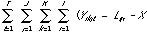
Cash flows and timber flows could be considered in the light of cumulative curves of procurement costs. Previously, Korpilahti [19] employed this curve as a useful tool when he illustrated the cost accumulation in wood procurement. In this application, the real, dynamic path of the capital accumulation for timber flows was approximated by the separately straight curve (Figure 4), which supported DMG's DM. Further, the graphs of cumulative cost curves were a presentation technique, which were used to analyze the hypothesis. By the graphs the separate cost effects on total and unit costs between the functions could be presented. A graph also provided an analysis of the internal adjustment process of the system, when the differences of the capital accumulation for two decision alternatives of the GDDM were described during the interval [t0, tn]. Solutions were provided by the following difference equation (or recurrence relation) [26].
where
Q(t) is capital accumulation during a time horizon (weeks' 36,...,43),
Q(ti) is capital accumulation at a selected discrete time (week's 36, 37,...,43),
dt is a derivative,
Dti is a change,
a is week number 36,
b is week number 43, and
n is number of discrete times.
The summation expression bears a certain resemblance to the definite integral expression. When the change in time is infinitesimal, the upper limit of the summation sign is infinite, and the integral is the continuous counterpart of the discrete concept of summations. However, models of this study dealt with discrete time when the volumes of decision variables were solved. Further, the variable t changed from one integer value to the next. For the graphs, timber-flow functions (stages) were described separately as four periods and by the average values. Therefore, the graphical expression was the separately straight curve.
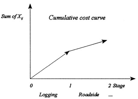
Figure 4. A cumulative curve is separately linear
RESULTS
Table 1 and Figure 5 show that there can be the different allocations of timber inventory resources between the conventional and local models when the system is the same and the DMG's goals are the same at both hierarchical levels. The allocations of the logging and transportation functions also changed, especially because the dynamics of the system were modelled by the dynamic balance equations and local time variable parameters (dynamic component). Consequently, the allocation costs were related to each other by the timber-flow functions which also influenced the adjustment costs of the fixed capital.
The local dynamic component caused a small margin (less than 1%) with respect to the conventional model. The allocations changed more clearly when the DMG set their own local goals of the roadside inventory at the beginning of the GDDM. The GDDM component caused the significant difference of the total costs between the initial models, which was about 24.6% (Table 1). Evidently, the different allocations resulted in the lower total costs when the local models and GDDM were used.
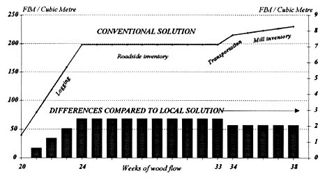
Figure 5. The cumulative curve of unit costs for the conventional model of the FDDM (left vertical axis) and the differences of the dynamic component when compared to the respective but lower costs of the local model of the FDDM (right vertical axis).

Display large image of Table 1
Table 1. Optimal solutions of the initial DLP models.
The hypothesis was investigated by comparing the results provided by the initial models with the results provided by the final model; comparison included the versions for the interest rate of 10%. First, the effects of the time factor were analyzed by the graph of the cumulative curves for total costs when the change of the buffer stocks of the stands was essential for feasible solution (Figure 6). The duration of stand inventorying (time factor) was meaningful, and influenced the total costs of timber procurement. Further, it seemed that the costs were affected by the capital accumulation and the interest rate (time factor) when they were included and considered as parts of cash flow. Obviously, the greatest proportion of the increases of the total costs were caused by the bigger procurement volumes during the DM horizon. This was evident and did not verify the hypothesis, but the shape of the curves did, because it revealed that the change of the time factor caused the dependence of the total costs.
Secondly, the specific analysis of the time-factor was provided by consideration of the internal adjustment process of the system (Figure 7). Both curves described cumulative differences of the unit costs (cost addition) between the initial model and the final model, from which the differences between the shapes of the total cost curves of Figure 6 were derived. At the end of the first stage of timber flows (logging), the cost difference of the total cumulation without interest was about FIM 3, while at the last stage of timber flow (mill inventorying) it was only FIM 1.5. The change for the diminished standing buffer caused these differences by the cost effect of combined logging costs and the final remittance of the stumpage price.
The effect of the time-factors was more evident when the correspondence of the differences of the unit costs (internal adjustments) was considered for the conventional model and the local model (Figure 5) versus the initial models and the final models (Figure 7). In both figures, the first models had conventionally determined (average) logging costs. In Figure 5 the costs of the second model were the local and time variable costs based on the FDDM. In Figure 7, the costs of the second models were the local and time variable based on the GDDM, i.e., the final solution was influenced by the more numerous time factors. In Figure 7, the peak of the difference value in week 16 compared to the value at the last stage of timber flows indicated the effect of the time-factors. The effect was about FIM 1.5, while the corresponding change from week 24 to week 38 in Figure 5 was about FIM 0.5.
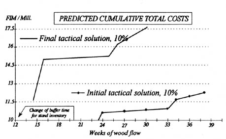
Figure 6. The time factor influenced strongly the total costs during the GDDM, when buffer stocks of standing inventories were changed from 20 weeks to 12 weeks.
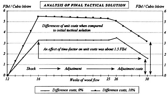
Figure 7. The analysis of the effects of the dynamic component in the GDDM was provided by consideration of the internal adjustment process; cumulative differences between the unit costs of the initial solutions and the final solutions are described by the curves.
DISCUSSION
The new synthesis was defined using the local planning goals of the tactical manager, which were assumed to be consistent with real-life requirements. Therefore, if these goals are fulfilled, then the GDDM is a useful tool to be implemented in solving practical problems. The validity of local models has already been discussed by Palander [25], and observed to be logical. Furthermore, the use of the dynamic approximation of the difference equation has also been observed to be logical [19, 24, 25]. However, the use of these tools is a part of the DM process. Therefore, considering the validity of the DDM techniques, this was also essential.
There are various reasons for the GDDM. The most important one was the well-defined structure of combined interior information flows. In the FDDM, information flows to the mills were only connected through the upper hierarchical levels, so that a more aggregated multi-level technique provided the framework for the DM process. Consequently, the term multi-level planning has been employed to describe functionally decentralized planning [17]. These techniques have been labourious to use and often they have lacked the communication tools to make them suitable for practical purposes. In the GDDM communication was natural because the DMG was small and permanent. Further, although the concrete coordination of DM of the DMG was assigned for themselves (supervisor), the management operations were strictly based on the manageable negotiation and optimization program. Therefore, what may be called information cheating [2, 15] can be controlled and avoided.
For the modelling of the system the FDDM has some serious disadvantages against the GDDM. In real life situations, the actors (employees, units) of the functional organization need more often to use cross connections outside the company's approved information flows. Further, cost responsibilities are not so self-evident as they should be in the local profit units. These non-descriptive characteristics of the FDDM make it mathematically more difficult to model, since the system has more unpredictable relationships between its elements. Furthermore, the huge running and replacement costs of programs of large-scale models have been a serious limitation for the more advanced use of FDDM. Therefore, the programs have been run only in centralized computer systems.
When the GDDM is used, programs for local management can be simpler and can use less computer memory. Consequently, configurations for PC computers become more feasible. As a further point, the cost of information exchange might be decreased by this technique for the reason that independent profit units could use a new strategy of information systems [29]. Of course, there could be other applications to responding to the GDDM and there could also be different system descriptions, which could be formulated as DLP models. In this context the discussion of the dynamic system is emphasized. For the dynamic balance of our models, the linking variables were the roadside and mill inventories. This decision was based on the dynamic structure of the system as described in Figure 3. Probably, there could be other possible choices for model construction, e.g., one or other from the timber procurement functions.
After numerous tests and the theoretical model considerations, however, it was difficult to imagine more appropriate and effective linking variables for dynamics than inventories. Moreover, the local managers' goals, the budget restriction and the buffer stock equations were linked by them. According to Hadley [12], the selection of state parameters of dynamic programming (DP) is a most subtle task. Once this is accomplished, it is usually a straightforward matter to obtain the dynamic recurrence relation. This is consistent with the results of our DP analysis [24] and was also observed in this study when the equations for dynamics of DLP (or states) were constructed between the periods. Therefore, sufficient time should be devoted to this phase of model construction.
Most often tactical decisions are related to time. Therefore, special considerations were concentrated for this aspect of the GDDM. The effects of the time factor were divided into partial sub-factors (capital, interest, logging costs, and transportation costs), described as functions of time. By using the model's time-varying cost parameters as the weights of the decision variables, three latter sub-factors had their combined cost effect (1%) of the total costs. This result agrees with the previous results presented by Palander [24] in the Table 5 for the unit costs of logging and purchasing. In that study the unit cost was described by the addition of logging of 10% for every week of the diminished standing buffer.
However, this cost effect was small. Given all the uncertainties, unknowns, and inaccuracies of data it is likely that a 1% difference is meaningless, and the two models perform the same when measured by the objective function. In our experiment of the GDDM were two of the system's elements of the first sub-factor (stand inventory, roadside inventory), which described the durations of the timber-flow functions. Roadside inventories were used to determine the effect of the GDDM component on the total costs of the initial model. The different local goals of the districts shortened the average duration of the roadside inventory. Therefore, the GDDM component caused the significant difference (24.6%) between the FDDM and the GDDM. Accordingly, the initial model based on the GDDM could be more accurate.
By using the buffer stock parameters as the RHS values of the constraints (goals), the effect of the first sub-factor on the total costs and the unit costs of the final model could be brought up during the GDDM. In addition, it is not necessary that decision makers set preference weights and goal levels in advance. Therefore, the instrumental theory of the parametric DLP may also be assumed to be appropriate for applications in extended systems of wood procurement. An example for successful consideration was the change of the volume of the standing inventory, which was caused by the requirement of the change of the buffer stocks. When the buffer stocks, as a defined time factor, diminish, the system's timber resource stock accumulates less capital for actions (timber flow) and the new state is closer to the JIT inventory.
The JIT inventory is a good aim when the state of the dynamic system is solved. Momentarily, however, the regional timber order increased and the mills' timber demands remained constant. Therefore, the stock, i.e., as the timber inventory on hand, and the total costs increased. The interpretations of the total cost curves seem to support the hypothesis, which assumes that the use of the dynamics is important in the GDDM. The results revealed that the time factor influenced the local total costs, although all aspects of the time factor from which the differences between shapes of total cost curves could be derived were not analytically defined through the results of this study. However, the dynamic component analyzed after the increase in the local resource stock (capital) was a shock for the dynamic system. Adjustments were tried and the situation was almost normalised by the new timber allocations. However, higher unit costs remained at the last stage of timber flows, which can be imagined to be the additional cost of the disturbance. For practical purposes, finding out the durations of timber-flow functions when there would be no additional costs in a system would be interesting. Then, the dynamics of a system could be controlled for balancing timber flows.
The cumulative curve was the useful tool for the analyses of the change of the costs. It had only the limitation of the linear assumption for its separate stages of timber flow, because the models dealt with discrete time and its average stage costs, i.e., the volumes of decision variables were determined separately, when time changed from one integer value to the next. It is also meaningful to see that the pattern of change in the variables was described by partial derivatives or differences, rather than by derivatives or differentials. In accurate graphical expressions, there could be knees in the 'stages' of the cumulative curve. Then the stages could be different from the separately straight cumulative curve. Furthermore, the curve could no longer be smooth as would be the case with non linearity.
In Finland, the organizations of the forest industry are changing, having fewer working managers, and the privately owned local timber-procurement enterprises are coming. Moreover, timber growing enterprises and procurement enterprises may soon form geographical integrations. Accordingly, their procurement will be controlled by the geographical delivery of contracts. This study provides some directions for management of local contractors, but more information about the geographical and participative techniques of the tactical DM is needed. Keipi [17] has described three styles of leadership based on Tannenbaum and Schmidt [30], which are suitable for participative DM:
Kilkki [18] has presented an example of the first alternative concerning a timber growing enterprise. The second style has been considered by Keipi [17] concerning functionally decentralized timber procurement planning. Based on this study, the third alternative is proposed, which may be the potential alternative for the GDDM in real life situations of the future.
REFERENCES
[1] Bailey, G.R. 1973. Wood allocation by dynamic programming. Canadian Forestry Service, Ottawa, ON. Publication No.1321.
[2] Baron, D.P. 1972. Joint decision technologies with a production marketing example. In: Tuite, M.F., Chisholm, R.K. and Radnor, M. [Editors]. Interorganizational Decision Making. Aldine, Chicago, Ill. P. 162?176.
[3] Clifton, R.G. 1989. JIT: Fad or future fact? Industrial Distribution Vol. 78 (June).
[4] Daugherty, P.J. 1992. Credibility of long-term forest planning: dynamic inconsistency in linear programming based forest planning models. University of California. Berkeley. [PhD Dissertation.] 167 p.
[5] Dykstra, D.P. 1976. Timber harvest layout by mathematical and heuristic programming. [PhD Dissertation.] Oregon State University. Corvallis. 299 p.
[6] Dykstra, D.P. and J. Riggs. 1977. An application of facilities location theory to the design of forest harvesting areas. AIIE Transactions 9(3): 270?277.
[7] Erdle, T.A., P.A. Arp and C.-H. Meng. 1982. Optimizing pulpwood inventories at roadsides, millyards and concentration yards: a case study. Proceedings of IUFRO S3.04.01. XVII World Congress. Kyoto. Japan. Sept. 6-17, 1981. Univ. of Maine. Misc. Rep. 264:40?51.
[8] Eskelinen, A. and J. Peltonen. 1977. Puunhan-kinnan suunnittelumalleilla suoritettava raakapuuvarastojen koon optimointi. [Optimization of the size of roundwood storages performed by logging planning models.] Metsäätehontiedotus 343. 29 p. [In Finnish with English summary.]
[9] Field, R.C., P.E. Dress and J.C. Fortson. 1980. Complementary linear and goal programming procedures for timber harvest scheduling. Forest Science 26:121?133.
[10] Galbraigth, J.E. and C.-H. Meng. 1981. Simulating optimum inventory of harvested wood. Journal of For. 79(5):292?295.
[11] Goulet, D.V. 1979. Tree-to-mill forest harvesting simulation models: where are we? For. Prod. J. 29(10):50?55.
[12] Hadley, G. 1964. Nonlinear and dynamic programming. Addison-Wesley Publishing Company. Inc., Reading, MA. 412 p.
[13] Hay, E.J. 1990. The just-in-time breakthrough. Implementing the new manufacturing basics. John Wiley and Sons. New York.
[14] Hotvedt, J.E., W.A. Leuschner and G.J. Buhyoff. 1982. A heuristic weight determination procedure for goal programs used for harvest scheduling models. Canadian Journal of Forest Research 12:292?298.
[15] Jennergren, L-P. 1972. Studies in the mathematical theory of decentralized resource allocation. The Economic Research Institute of the Stockholm School of Economics, Stockholm. 171 p.
[16] Keipi, K. 1977. Transfer pricing for log allocation in a decentralized forest products firm. Helsinki. Commun. Inst. For. Fenn. 89(2):1?114.
[17] Keipi, K. 1978. Approaches for functionally decentralized wood procurement planning in a forest products firm. Helsinki: Commun. Inst. For. Fenn. 93(4):1?116.
[18] Kilkki, P. 1987. Timber management planning. University of Joensuu Faculty of Forestry. Silva Carelica 5:1?160.
[19] Korpilahti, A. 1990. Puunhankinnan kausi-vaihtelun vaikutuksesta puuvirtaan, resurssien kääyttöööön ja
hankintakustannuksiin. [On the Effects of Seasonal Variation in Wood Procurement.] Metsäätehontiedotus 404. 19 p. [In
Finnish with English summary.]
[20] Lohmander, P. 1989. Stochastic dynamic programming with a linear programming subroutine: Application to Adaptive Planning and Coordination in Forest Industry Enterprise. Swedish University of Agricultural Sciences. Dept. of Forest Economics. Rep. 93. 51 p.
[21] Lohmander, P. 1991. The optimal dynamic production and stock levels under the influence of stochastic demand and production cost functions: theory and application to the pulp industry enterprise. Swedish University of Agricultural Sciences Dept. of Forest Economics. 138 p.
[22] Lohmander, P. 1992. Decision optimization with stochastic simulation subroutines: relation to analytical optimization of capacity investments and production. Swedish University of Agricultural Sciences Dept. of Forest Economics. Rep. 148. 51 p.
[23] Mikkonen, E. 1983. The usefulness of some techniques of the mathematical programming as a tool for the choice of timber harvesting system. Acta For. Fenn. Rep. 183. Helsinki. 110 p.
[24] Palander, T.S. 1995a. A dynamic analysis of interest rate and logging factor for reducing saw timber procurement costs. Journal of Forest Engineering 7(1):29?40.
[25] Palander, T. 1995b. Local factors and time-variable parameters in tactical planning models: a tool for adaptive timber procurement planning. Scand. J. For. Res. 10:370?382.
[26] Petkovsek, M. 1991. Finding closed-form solutions of difference equations by symbolic methods. [PhD Dissertation.] Carnegie-Mellon University. 124 p.
[27] Porter, M.E. 1980. Competitive strategy. Techniques for analyzing industries and competitors.
[28] Rowland, J.R. 1986. Linear control systems. Modelling, analysis, and design. John Wiley and Sons. 511 p.
[29] Scheer, A.-W. 1989. Enterprise ? wide data modelling. Information systems in industry. New York Springer.
[30] Tannenbaum, R. and W.H. Schmidt. 1958. How to choose a leadership pattern. Harvard Business Review. Vol. 36(2):95?101.
[31] Seppäälää, R. 1971. Simulation of timber-harvesting systems. Folia Forestalia. 125. Inst. For. Fenn. Helsinki. 36 p.