July, 1998, vol.9 no.2
L.G. LeBel
Université Laval
Québec, Canada
W.B. Stuart
Virginia Polytechnic and State University
Blacksburg, USA
The authors are Professor of Forest Operations and Professor of Industrial Forestry Operations respectively.
ABSTRACT
Data Envelopment Analysis (DEA) models were used to measure the technical efficiency of a sample of logging contractors. DEA is a nonparametric efficiency measurement technique based on linear programming methods. This paper demonstrates how DEA models can be applied in a forest operations context to gain insights on the factors which affect technical efficiency and performance.
Twenty-three fully mechanized loggers were compared in regards to the efficiency with which they converted inputs - dollars of capital, consumables, and labor - into output - tons of wood. Overall, for the period of 1988 to 1994, the logging contractors studied were efficient, but some were considerably less efficient than others. Low capacity utilization had a negative impact on technical efficiency. The scale of an operation also influenced technical efficiency. For the sample, the most productive scale size was estimated to be around 75,000 tons per year.
Keywords: Forest harvesting, Data Envelopment Analysis (DEA), efficiency.
INTRODUCTION
In forest operations, performance is frequently rated on the basis of common sense or past experience [22]. While sufficient in many instances, the complexity of today's business environment and harvesting systems are such that a more precise method must be applied. Precision is particularly important in periods when technological improvements are achieved at an increasing cost. Carter and Cubbage [7] identified technical change as a main source of efficiency improvement between 1979 and 1988 - a period during which many southern firms switched from shortwood to longwood systems. Now that the technology has stabilized, it appears increasingly evident that significant gains in efficiency could also come from a better understanding of the "soft" components of the wood supply system. Such components include capacity utilization, contractor's zeal, procurement organization's philosophy, and governmental regulation. By understanding how these factors affect technical efficiency, it may become possible to improve the efficiency and performance of individual contractors and the wood supply system as a whole.
Askin and Standbridge[3] define effectiveness as doing the right task, efficiency as doing a task right, and performance as accomplishing the right task efficiently. Sink and Tuttle[21] maintain that system performance is a function of the complex interactions among seven criteria. These criteria are efficiency, effectiveness, quality, productivity, quality of work life, innovation, and profitability. The research presented here focused on technical efficiency for two reasons. First, efficiency is a prerequisite of operational performance. Second, it is one of the most objectively quantifiable dimensions of performance, making it relatively easy to be agreed upon.
This study had two main objectives: 1) to develop an analysis tool that would properly assess costs and production information and compute technical efficiency ratios, and 2) to increase the understanding of the logging contractors' business environment by identifying the factors which contribute to technical efficiency and business performance.
EFFICIENCY MEASUREMENT
Technical efficiency can be expressed as the ratio of what a production unit produced over what it consumed. A measure of relative technical efficiency can be obtained by comparing production units against a common standard. The efficiency standard must be estimated since one usually has experimental observations only and does not know the exact shape or location of the production frontier [1]. The difference or distance between an observation and the production frontier provides a measure of inefficiency[9]. The ability to specify a best practice standard is a prerequisite to technical efficiency measurement.
Efficiency measurement techniques can be divided into two groups depending on how the production function is estimated. Parametric models, such as the Ordinary Least Square (OLS) and the stochastic frontier approach have been applied in forestry[7]. Nonparametric models such as DEA have seen increasing interest in recent years [23] but had yet to be applied to forest harvesting.
Data Envelopment Analysis (DEA) uses linear programming to compute a hull that envelops all the data points by linking the most efficient observations. The hull is referred to as the empirical production function as it is based on actual observations [1]. The distance between the envelope and an observation is computed to provide a measure of Farrell's technical efficiency [9]. The approach should be intuitively appealing to managers because the envelope defines a standard based on actual observations - real loggers - and not a composite operation based on statistical manipulation. As a nonparametric method, DEA requires no assumption regarding the statistical distribution of the efficiency scores. More over, it is not necessary to assume that all observations, also referred as Decision Making Units (DMUs), share a common and identical production function [6].
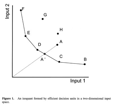
The DEA methodology is illustrated in Figure 1 for a group of production units using two inputs. The best-practice frontier is defined by literally "enveloping" all DMUs. The model defines an isoquant by linking DMUs B, C, D, E, and F. Those are considered to have a relative efficiency of one, or 100%, as they lie on the production frontier. The less efficient units (A, G, H) lie inside the isoquant.
A measure of radial efficiency is computed by comparing the inefficient unit A with an efficient one located where the ray OA intersects the isoquant (A'). A' is obtained from a weighted combination of neighboring observations on the isoquant (D and C). DMU A is less efficient than A' since it is using proportionally more of both inputs to produce the same quantity of output. The rationale for taking radial measurements is to insure that the peer unit selected uses inputs in the same proportion as the inefficient observation. This is to reflect management values or environmental constraints that may have restricted input substitution.
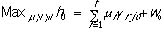
Charnes et al.[8] specified a fractional linear program that computes the relative efficiency of each DMU by comparing it to all the other observations in the sample. The approach, known as the CCR model in reference to its authors (Charnes, Cooper, and Rhodes), attempts to maximize the ratio of the weighted outputs over the weighted inputs, subject to the constraint that no other DMU has a ratio h0 larger than one when using the same weights.
Model 1

subject to
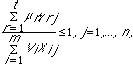
where
yrj = amount of output r produced
by unit j,
xij = amount of input i used by unit j,
µr = the weight given to output r,
Vi = the weight given to input i,
n = the number of DMUs in the data set,
t = the number of outputs,
m = the number of inputs,
e = infinitesimal, e>0 (a small positive number).
The justification for e is twofold [27]: first, to ensure that the denominator is never zero. Second, and this is more of a managerial concern, to ensure that each input (output) is considered. It is simple to transform Model 1, a fractional linear program, into a linear program (Model 2) which can be solved with the simplex algorithm:
Model 2
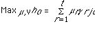
subject to
In their initial formulation Charnes et al. [8] assumed constant returns to scale when comparing observations of different size. In Model 3 Banker et al [5] relaxed this assumption by adding the unrestricted multiplier w to consider cases where variable returns to scale are present. The model is often referred as the BCC formulation in reference to its authors (Banker, Charnes, and Cooper).
Model 3
subject to
W0 unconstrained in sign.
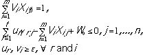
Figure 2 was adapted from Banker et al [5] to illustrate the difference between technical, scale, and aggregate efficiency. The production frontier estimated by Model 2 would be the straight line OD because of the constant returns to scale assumption. Unit D has the largest average productivity of all units in the set, and it is the only DMU deemed fully efficient. By comparison Model 3 defines the line BCDE as the best-performance envelope. When measured with the BCC model efficiency is referred as technical efficiency, or "pure" technical efficiency by some authors [5]. Aggregate efficiency, as measured with Model 2, has a scale and technical components. Units B, C, and E were deemed efficient using Model 3 because it does not consider scale inefficiencies. It is possible to isolate scale efficiency by taking the ratio of aggregate efficiency (Model 2) to technical efficiency (Model 3).
For example, unit A is inefficient: for a same level of output, unit B uses fewer inputs, or, alternatively, unit A produces less output than unit C while using the same level of inputs. The fraction MB/MA measures the technical efficiency of unit A. The product of pure technical and scale efficiencies, MN/MA, is a measure of aggregate efficiency. MN/MB is a measure of scale efficiency for unit A and can be obtained by dividing Model 3 by Model 2: MN/MA÷÷MB/MA = MN/MB.
Without the convexity constraint of Model 3, unit A would be compared with the composite unit "N," a linear extrapolation based on the average productivity of a unit located at the most productive scale size - unit D. Model 3 allows for a better "fit" to the observations by forcing peer units to be of comparable size to the inefficient DMU. A drawback of using a variable scale model which offers a better fit is in the higher number of unitary-efficient DMUs obtained, i.e., observations on the envelope. Weight restrictions allow the analyst to restrict the "region" of full efficiency, therefore reducing the number of unitary-efficient observations. The reader should refer to Roll et al. [18], and Allen et al. [2] for a complete description of weighting procedures. Also, Shiba [23] provides useful insights specific to DEA's possibilities in a forest management context.
METHODS
The work of several researchers [25,12,14], spanning a period of six years, has resulted in one of the most up-to-date and detailed cost and production information sources on southern logging operations. Each of the contractors involved in the study was visited several times to observe the work environment and the equipment in use. On-site discussions also provided insights concerning each contractor's business background, management style, and strategic planning. Six years of cost and production data were collected from a group of 23 loggers providing a total of 109 logger-years.
The median annual production for the complete sample is 63,665 tons of round wood. The largest contractors produced 237,672 tons, and the smallest produced 21,373 tons. Business expenses were divided into three broad categories - Capital, Consumables, and Labor, that accounted for over 90% of all logging costs. Capital includes investments in depreciable assets, rent, lease, licenses, and taxes. Consumables are supplies that are expended in the short term. It includes repair and maintenance supplies, parts, fuel, oil, tires, tubes, and saw expenditures. Labor is comprised of all items related to employee compensation (salary, wage, workers' compensation insurance, employee benefits). The median value for capital, consumables, and labor expenditures is $182,314, $205,982, and $320,917 respectively. Technical efficiency was evaluated based exclusively on the loggers utilization of these three economic inputs.
No adjustment for inflation was made despite the fact that financial information ranging from 1988 to 1994 was used. It was found difficult to obtain the proper index that would take into account regional differences in prices, and improvements in machine productivity and reliability. Moreover, it was in part the purpose of the study to identify the effects of price changes on efficiency over time.
Data envelopment analysis offered interesting potential to extract as much information as possible from such a large data base. The DEA models were coded on Mathematica® for Windows® [12,26]. Mathematica appeared well-suited to handle the computation-intensive linear programming models. In their final form, the DEA models are transparent and it is easy for the user to modify or add subroutine to the software.
Radial efficiency measures were taken, first with the CCR model to provide an "overall" or "aggregate" measure of technical efficiency, then with the BCC model to provide a measure of "pure" technical efficiency. Finally, non-radial measures [10] were taken to estimate the efficiency with which each input factor was utilized (partial efficiency). Partial efficiency measurements provide information regarding the rate at which each input factor is transformed into output.
The eventuality that some technological development has occurred must be carefully investigated when a study extends over such a long time horizon so as not to confuse progress owing to technical efficiency and technological progress [19]. Carter and Cubbage [7] reported an annual average technical change of 1.8% between 1979 and 1987. In the South, this period was characterized by increased tree-length harvesting and major technical improvements in regards to felling machines and grapple skidders. Fewer significant technological developments took place since data collection began in 1988. Nevertheless, changes in the southern procurement system have occurred and were considered. For example, wide-tired skidders and tracked feller-bunchers have become more prevalent. These changes in technology largely reflect efforts to comply to the more restrictive environmental regulation and are suspected to have had a significant influence on the efficiency of some contractors.
RESULTS AND DISCUSSION
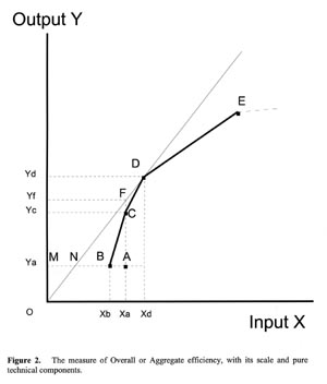
The mean overall efficiency (CCR) for the sample was 79%, while the mean pure technical efficiency (BCC) was 84%. The median was 82% and 86% for the CCR and the BCC respectively. Both efficiency distributions had a standard deviation of 0.13.
When efficiency scores were segregated on an annual basis, the DEA models revealed a radical decrease in technical efficiency in 1990 (Figure 3). Technical efficiency continued to decrease slightly until 1994 when it rebounded. In the late 1980s, loggers were hard-pressed to keep their costs at a minimum and many were living off their equity [14]. After a difficult year in 1990, during which production fell, loggers were unable to achieve high efficiency despite increased production volumes. Reasons for this varied among contractors. Some were updating their equipment spread, causing their capital efficiency to drop. Some were working on tracts that required considerable increases in consumables. Others were impeded by quotas from producers.
Non-radial models are necessary to compute partial efficiencies and learn more about the possible causes of efficiency variations. The Asymmetric-Fääre (AF) model [10] was used to measure partial efficiency (Table 1).
Table 1.
| Capital | Asymmetric-Faare Consumables | Labor | |
| Mean | 0.55 | 0.72 | 0.81 |
| Median | 0.44 | 0.67 | 0.84 |
| 25th Percentile | 0.33 | 0.54 | 0.71 |
| 75th Percentile | 0.76 | 0.88 | 0.94 |
With the AF model, each input is scaled down, in turn, to the envelope while holding the other inputs constant. Contrary to radial measurements, partial efficiencies are based on the premise that contractors could have substituted inputs and changed the proportion in which they used them.
Average partial efficiency was the lowest for capital. It can be observed from the median, first, and third quartile values that the distribution of capital efficiency was not symmetrical. Only a few loggers enjoyed high capital efficiency, and were on or near the envelope, while a majority fell far from the frontier. On average, capital efficiency plummeted in 1990 and remained low for the rest of the period studied.
Two approaches were identified among loggers with high capital efficiency. Some were using depreciated equipment. Others, while using newer equipment, did not have to carry excess production capacity.
Consumables efficiency also dropped in 1990. Among possible explanations are the increased use of high-flotation tires on skidders and feller-bunchers, and a switch made by some loggers from tire-mounted to track-mounted felling machines. These efforts to reduce site damage contributed to lower technical efficiency.
Most loggers achieved comparable efficiency level in their application of labor. This is partly due to the fact that all contractors used similar equipment with similar labor requirements, and all have to comply to strict federal and state regulation. Yet, two clusters were identified: those observations which lay below a labor efficiency of 0.70, and those which lay above. There were three threads linking the lower observations: 1) low capital input, which may indicate older equipment requiring frequent repairs; 2) family operations, which tended to have more generous compensation packages; 3) higher volume of hardwood, which often requires more of all inputs.
The implication of varying logging capacity utilization was studied. A statistically significant correlation was found between capacity utilization and technical efficiency: periods of low capacity utilization tended to have a lower overall efficiency score. The relationship between capacity utilization and partial efficiencies indicated that, at least for some loggers, labor costs are not as variable as many may expect. During periods of low production, some loggers were not in a position to reduce labor costs sufficiently to remain technically efficient. Loggers avoid temporary layoffs because they lead skilled workers to look for employment elsewhere. In the past labor could find temporary employment on farms, or remain idle during layoffs. Today's qualified operators demand permanent employment.
Managerial strategies regarding labor and capital utilization only account for a fraction of the factors determining efficiency. Exogenous factors to which contractors must continuously adapt were considered.
The Work Environment
The three factors that had the greatest effect on technical efficiency were hauling distance, percentage of hardwood in the tract, and capacity utilization. A worse case scenario would be for a logger to have a low producer quota while working a hardwood tract on a long haul. In most cases the combined effect is not that dramatic. These factors' direct actions and interactions could warrant a further investigation in their own right [12,15,16]. For the purpose of this study the factors were considered as a whole in an attempt to properly mirror the working conditions. This was achieved through a "complexity factor" developed to account for their combined impact and to provide a surrogate of the working environment [13].
The complexity factor assigned equal weight to each of the three variables and served as a "difficulty rating." The higher the complexity factor, the more difficult the working environment for a particular operation.
The Spearman's coefficient of correlation between the complexity factor and three performance criteria was computed. Loggers with a high complexity factor, i.e., more difficult tracts, tended to have a lower technical efficiency rating (p <0.01). The cost per ton rose with an increase in the complexity factor (p <0.001) while production showed no significant correlation (p = 0.68).
These figures should certainly not be interpreted to imply that production cannot be affected by tract conditions. Rather it only suggests that the contractors included in the study were able to adjust their input utilization level to maintain their targeted production. On a difficult tract, a logger would consume a higher level of input just to maintain production. On more favorable tracts, a logger may not increase production as much as one may expect - sometimes because of quotas -but the level of input required is generally reduced and efficiency is increased. To a certain degree, contractors can adapt their system and maintain a given output level for a wide variety of tract conditions. This degree of adaptability was referred to as "production elasticity" [14]. In the South, production elasticity is often a required performance characteristic for a contractor despite its potential impact on technical efficiency. The true value of production elasticity must therefore be considered from a financial perspective.
Technical Efficiency and Financial Margin
The ultimate goal of a business is the preservation and growth of equity [24]. Maximizing profits contributes to the preservation and growth of equity. On the other hand, striving for maximum technical efficiency, especially if it means minimizing cost, does not guarantee profit maximization: they are often considered separate objectives. The relationship between technical efficiency and financial margin was explored.
The most productive scale size (mpss) is the point where a contractor achieves highest technical efficiency [4], minimizes average unit cost, and maximizes unit margin. By definition, this point is only achieved by loggers who have an aggregate efficiency of one. All other DMUs have more or less deviated from the mpss and have a certain degree of scale inefficiency. In the sample, an average of 26% of all inefficiency was scale related. Certainly there are forces and motivations leading contractors to stray from the mpss.
Firms in a competitive market optimize their total margin by producing the quantity of output at which the rate paid equal to the marginal cost of producing that last unit [17]. Such a production size is usually located past the point of minimum average cost. Unlike the mpss, which is independent of the rate paid, the most profitable level of operation is dependent on the rate paid per unit. Loggers will move away or closer to the point of maximum technical efficiency depending on the price they receive.
The data provided the opportunity to track how operation size, profit, and efficiency are interrelated. First, it was important to link differences in revenues to differences in scale efficiency without the "noise" introduced by technical inefficiencies. Accordingly, only loggers with a pure efficiency (BCC) above 90% were selected so that scale penalties would be isolated. Based on these data, an equation of cost as a function of annual production was generated (Eq. 1).
Eq. 1
C = 0.00003x(P)2 + 5.0785x(P) + 144,348
r 2 = 0.986
where
C = Total operating cost,
P = Annual production in tons.
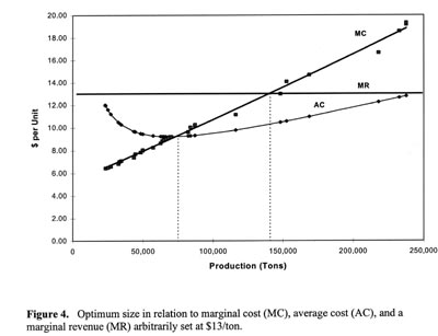
The average and marginal costs were computed based on that function and are plotted in Figure 4. It can be observed that average cost is minimized at a production size near 75,000 tons. The AC curve reflects the presence of increasing returns to scale up to that size, and decreasing returns afterward. Total margin, however, increases as long as marginal cost (MC) is smaller than the rate paid (MR). For example, if the rate paid is $13 per ton (marginal revenue), loggers would benefit from expanding production up to a volume of approximately 140,000 tons.
If a rate just equal to the lowest average cost per unit is paid loggers are forced to maximize overall efficiency because scale inefficiency would erase profits. Consequently, for a comparable technology, loggers would converge to a similar operating size. No elasticity is then available since no matter what direction a logger's production goes, up or down, average cost increase and profitability is reduced. For every dollar paid above the minimum rate, a procurement organization "buys" more production elasticity. Based on the most efficient loggers in this study, a rate of $12 per ton would allow for a wide range of profitable operating sizes - from 25,000 to 250,000 tons.
The relationship between aggregate efficiency and total margin is different depending on whether a logger is to the right or left of the mpss. Striving for better overall technical efficiency is legitimate for small loggers producing to the left of the minimum average cost as they increase their unit and total margin. For example, contractors increasing overall technical efficiency and production from 25,000 tons to 75,000 tons increase their margin (both unit and total). But once past the mpss, near 75,000, overall technical efficiency decreases, and total margin increases until marginal cost equals marginal revenue. Larger contractors who are on the upward sloping side of the average cost curve have sacrificed overall technical efficiency for larger overall profits.
In practice, this signifies that loggers placed on a 75% quota (relative to their regular wood orders) will experience a decrease in total and unit margin if they are located to the left of the mpss. Those located to the right will see a decrease in total margin but an increase in their unit margin and are more likely to remain profitable. Moreover, the slope of the AC curve is steeper to the left of the minimum cost point. Therefore, loggers to the left of the least cost point may expect their unit cost to change more drastically for a proportionate change in production compared to loggers to the right of the mpss. Many contractors appeared to be restricted to the negatively sloped section of the average cost curve by managerial and environmental factors.
For a given scale size, loggers with lower efficiency always have higher costs than the more efficient ones. The most BCC-efficient loggers have a lower average cost curve than less efficient loggers. For a given scale size, technical efficiency determines the average cost for a contractor; the less efficient, the higher the average cost. By controlling his efficiency a logger can influence his production cost. But for a same level of efficiency, management determines the level of operation along the average cost curve, and, indirectly, the logger's total margin. The ability of loggers to move along the AC curve while remaining efficient deserves further attention.
Loggers often move from periods of high efficiency to periods of lower efficiency as equipment is replaced or the working environment changes. Loggers who were able to spread their equipment renewal over time had a more stable efficiency from one year to the next. Many of the most stable loggers were identified as preferred suppliers. Their special status with the procurement organization allowed them to customize their logging operation to match the task expected of them. As a result, they usually enjoyed higher capacity utilization.
Elements other than the rate paid factor into the decision of a contractor to settle at a given operation size. The most obvious are weekly quotas, equipment financing, and tract size. Once regulated by quota a logger gains no advantage by increasing his scale as the quota would only be reached sooner. In regions where tracts tended to be smaller, operations were often of lesser scale. The discomfort of some procurement managers' in dealing with large operations may explain the high concentration of operations at or near an annual volume of 60,000 tons.
For the type of mechanized system included in this project, there is a production level below which contractors cannot justify the entry cost. Thirty years ago the entry cost for a pulpwood producer in the South was relatively low: a bob-tail truck, a pair of mules, and a bowsaw. Today, if mechanized felling and skidders are utilized, ownership and operating costs are substantial even for second-hand machines. Among those loggers closest to the entry point, the most efficient were all using depreciated equipment. Based on Equation 1 the aggregate fixed cost, or the minimum capital, required to enter mechanized logging is $144,348. This is approximately the capital value of a used equipment-based logging operation in the South. Within the smaller operations, reducing capital expenses to a minimum was the strategy adopted by the most efficient loggers. Labor efficiency tended to be lower for these operations as the burden of sustaining production was then transferred from equipment to the workers who were paid for idleness and maintenance work. In some market conditions, such as those encountered when recurrent quotas exist, this may be an appropriate strategy, but it will be increasingly difficult for small contractors to remain competitive if labor costs continue to increase.
CONCLUSION
DEA provided useful insights on the causes of efficiency variations in the logging contractor data set. In many instances it served to validate and quantify intuitive notions commonly held by contractors.
Overall efficiency was optimum near a production level of 75,000 tons per year. The DEA efficiency measures indicated that many of the smaller operations were inefficient and were likely to be in a precarious financial position, especially if new equipment was used. As long as the rate paid is higher than the marginal cost, a logger will always have the advantage to produce at a size larger than the mpss. In periods of low market demand, for example, quotas may be imposed and loggers may be forced away from the point of maximum total margin. In theory the same results could be achieved by reducing the rate paid, but then loggers operating on a narrow margin because of operational inefficiencies will move even closer to bankruptcy. If a procurement organization fixes its rate at or near the minimum average cost, the contractors will converge towards the mpss. The system will have no production elasticity; any increase or decrease in output will cause loggers to lose money.
High efficiency achieved sporadically may be less desirable than stability at a slightly lower efficiency level because it may indicate a lack of operational elasticity. Just as 100% capacity utilization is undesirable for a production unit faced with variations [11], 100% technical efficiency may not be in the system's best interest. In addition to cost considerations, the desired level of technical efficiency should reflect the environment, the procurement organization's need for flexibility, and stability in wood flow deliveries.
The reasons for which most larger contractors were experiencing decreasing returns to scale are not entirely understood. A detailed analysis of tax issues, overhead costs, and procurement issues such as tract size and administrative cost seems necessary. It does appear clear, however, that focusing on the least cost places even the most efficient contractors in a situation where any deviation from their production volume causes unit costs to increase.
LITERATURE CITED
[1] Ali, A.I. and L.M. Seiford. 1993. The mathematical programming approach to efficiency analysis. In: Fried, H. O., C. A. K. Lovell, S. S. Schmidt, eds. The measurement of productive efficiency: techniques and applications. New York, NY: Oxford University Press.
[2] Allen, R., A. Athanassopoulos, R.G. Dyson, and E. Thanassoulis. 1996. Weights restrictions and value judgments in data envelopment analysis: evolution, development and future directions. Annals of Operation Research.
[3] Askin, R.G. and C.R. Standbridge. 1993. Modeling and analysis of manufacturing systems. New York, NY: John Wiley and Sons, Inc.
[4] Banker, R.D., A. Charnes and W.W. Cooper. 1984. Some models for estimating technical and scale efficiencies in Data Envelopment Analysis. Management Science 30(9):1078-1093.
[5] Banker, R.D. and R.M. Thrall. 1992. Estimation of returns to scale using Data Envelopment Analysis. European Journal of Operation Research 62:74-84.
[6] Bernard, J., U. Cantner and G. Westermann. 1996. Technology leadership and variety: a Data Envelopment Analysis for the French Machinery Industry. Annals of Operations Research 68:361-377.
[7] Carter, R.C. and F.W. Cubbage. 1995. Stochastic frontier estimation and sources of technical efficiency in southern timber harvesting. Forest Science 41(3):576-593.
[8] Charnes, A., W.W. Cooper and E. Rhodes. 1978. Measuring the efficiency of decision making units. European Journal of Operational Research 2:429-444.
[9] Farrell, M.J. 1957. The measurement of productive efficiency. Journal of the Royal Statistical Society 120(3):253-281.
[10] Ferrier, G.D., K. Kerstens and P. Vanden Eeckaut. 1994. Radial and nonradial technical efficiency measures on a DEA reference technology: a comparison using US banking data. Discussion Paper, Universitéé Catholique de Louvain (CORE). Louvain-La-Neuve.
[11] Goldratt, E.M. and J.I. Cox. 1992. The goal: a process of ongoing improvement. Second revised edition. North River Press, Inc. 337 p.
[12] LeBel, L. 1993. Production capacity utilization in the southern logging industry. Blacksburg, VA: Virginia Polytechnic and State University. Thesis. 129 p.
[13] LeBel, L. 1996. Performance and efficiency evaluation of logging contractors using Data Envelopment Analysis. Blacksburg, VA: Virginia Polytechnic and State University. Dissertation. 201 p.
[14] Loving, R.E. 1991. Components of logging costs [thesis]. Blacksburg, VA: Virginia Polytechnic and State University. 204 p.
[15] Määkinen, P. 1992. Puutavaran kuljetusyrity-sten Menestymisen Strategiat [Strategies used by timber truck transport companies to ensure business success]. Acta Forestalia Fennica. The Society of Forestry in Finland/The Finnish Forest Research Institute. Report 238. [In Finnish, English summary.]
[16] Määkinen, P. 1993. Metsääkoneyrittäämisen Menestysyekijäät [Success factors for forest machine contractors]. Folia Forestalia. The Finnish Forest Research Institute. Report 818. [In Finnish, English summary.]
[17] Pindyck, R.S. and D.L. Rubinfeld. 1989. Microeconomics. New York, NY: Macmillan Publishing Company, NY. 668 p.
[18] Roll, Y., W.D. Cook and B. Golany. 1991. Controlling factor weights in Data Envelopment Analysis. IIE Transactions 23(1):2-9.
[19] Seaver, B.L. and K.P. Triantis. A fuzzy clustering approach used in evaluating technical efficiency measures in manufacturing. Journal of Productivity Analysis 3:337-363.
[20] Seiford, L.M. 1990. A bibliography of Data Envelopment Analysis (1978-1990). The University of Massachusetts. Amherst, MA: Department of Industrial Engineering and Operation Research.
[21] Sink, D.S. and T.C. Tuttle. 1989. Planning and measurement in your organization of the future. Institute of Industrial Engineers, Norcross, GA: Industrial Engineering and Management Press. 331 p.
[22] Sundberg, U. and C.R. Silversides. 1987. Operational Efficiency in Forestry. Kluwer Academic Publishers. Boston, MA. 219 p.
[23] Shiba, M. 1997. Measuring the efficiency of managerial and technical performances in forestry activities by means of Data Envelopment Analysis (DEA). Journal of Forest Engineering 8(1):7-19.
[24] Stuart, W.B. 1995. Unpublished. Logging Business Management. Workshop series. Blacksburg, VA.: Virginia Polytechnic and State University.
[25] Walter, M.J. 1996. Master thesis - Draft. Blacksburg, VA.: Virginia Polytechnic and State University.
[26] Wolfram, S. 1991. Mathematica: a system for doing mathematics by computer. 2nd Edition. Redwood City, CA.: Addison-Wesley Publishing Co.
[27] Wong, Y.-H.B. and J.E. Beasley. 1990. Restricting weight flexibility in Data Envelopment Analysis. Journal of the Operational Research Society 41(9):829-835.