
July, 1999, vol.10 no.2
Jimin Tan
The Australian National University
Canberra, Australia
The author is a Professor in the Department of Forestry.
ABSTRACT
The spatial and heuristic road locating procedure developed in an earlier study [16] has been improved and integrated using microcomputers. Further applications and results of testing the procedure using the same data are presented. The improved procedure proved to be beneficial in helping forest road planning managers evaluate alternatives and hence select the optimal location for a road network. It contains a heuristic algorithm capable of locating forest roads so as to minimise the total costs and impacts of road construction, wood extraction, and wood transport.
Keywords: Roads, location, net benefit, shortest paths, heuristic, microcomputers.
Introduction
Forest roads are built to provide easy access to the forest. In general, transport is cheaper by road than over forest terrain but the cost of building the road trades off against this reduction of cost. The forest road network should be located to minimise the total cost of wood extraction, wood transport and road construction, and to minimise adverse environmental impacts. Locating a forest road network is usually guided by optimising road spacing. Optimal road spacing is calculated as the break-even point between the road construction cost and wood transport cost [4, 6, 8, 10, 15, 13,18].
The difficulty in using an optimal road spacing method for locating forest roads is in taking into account the spatial diversity of forest stands and terrain conditions. Costs of transport and road construction vary with these factors. Location of the roads is not only governed by optimal spacing but also subject to restrictions dictated by the forest terrain. Optimal road spacing is therefore only a value that provides a guide for locating roads and a cost target but
does not suggest where the roads should actually be placed. It is therefore necessary to develop a road locating method that is capable of accounting for spatial variation of forest environments and resources.
A review of relevant literature was given in [16]. Seven articles in a recent publication [11] are directly related to computer supported planning of forest roads. Geographic Information Systems [1, 3, 14, 17] and Operations Research [5, 9, 12, 13, 18] are the main techniques used. The microcomputer procedure presented in this paper uses techniques of both Geographic Information Systems (GIS) and Operations Research (OR) to assist optimum location of forest roads, enabling consideration of the spatial variation of forest stands and terrain.
THE PROCEDURE FOR LOCATING A FOREST ROAD NETWORK
Road Location Aids
Practical procedures for locating forest roads may include many formal steps. Examples of such steps are shown in Figure 1. Steps 4 and 5 may be repeated until satisfactory results are achieved. Step 4 may begin with a simple survey such as checking certain critical points on the road route by walking into the forest and may subsequently involve a high level survey using a theodolite. The procedure developed during this study was aimed at assisting road-planning managers to determine the optimum location of a road network for a given forest area. The procedure provides two types of road locating aids as listed below.
(1) A costing and routing subsystem (CARS) was developed to enable a road-planning manager to evaluate alternatives of road network location and hence assist in determining the optimum location of a road network. [16] presented details of this subsystem, including spatial data representation and network formulation; minimum cost routing for wood extraction, wood transport and road construction. These modules have now been integrated in one program using a microcomputer. Only the spatial data handling process was implemented on a microcomputer in [16] and all other network modelling programs were carried out using a mainframe computer because of the high demand on computer resources. This change improves its user interface and makes it easier for users to generate road routes and compute their costs and benefits. The use of this subsystem for optimising the location of a road network will be demonstrated later in this article.
(2) A network extension tools subsystem (NETS) was developed to generate optimum location for forest roads serving a given forest area such that the total costs and impacts of road construction, extraction, and transport are minimised. Subsystem NETS must be used after subsystem CARS. In previous study [16], the optimum location of a forest road network was estimated using a heuristic algorithm. A recent development to this component was the solution of optimum road location using dynamic programming, which will be presented in another paper later. This paper focuses on the performance of the system using the heuristic procedure on a microcomputer.
Both subsystems were integrated and implemented using Visual Basic on a Pentium 100 MHz microcomputer. Their functions are summarised in Figure 2.

Spatial Data Representation and Minimum Cost Routing
To demonstrate how it can assist the location of forest roads, the essential functions of the CARS subsystem is described briefly, including spatial data representation, network definition and minimum cost routing.
In order to account for the spatial variations of forest environments and resources in locating forest roads, a spatial database is necessary. To represent spatial data, a coordinate system must be defined.
Figure 3 illustrates the uniform grid system which is used. The grid cells are spatially referenced by x and y coordinates. With the grid system, the coordinates are integers, rather than continuous quantities. For the convenience of computer output, the positive direction of y-ordinates is downwards while x-abscissa is positive to the right. For ease of referencing, grid cells have been sequentially numbered because it is more convenient to refer a grid cell by a single (sequential) number than that by coordinates (two numbers). The sequential number and coordinates of a cell can be linked as shown in Figure 3. Thus, a grid cell can be easily referenced and represented spatially by a single number.
If each of the grid cells is associated with expected cost values, the cost data can also be represented spatially. An example is shown in Figure 3, where average values for road and extraction costs are assigned to each cell. The quantity of transport is estimated in t/ha for every cell since it is a factor affecting the costs of extraction and transport. Each grid cell has dimensions of 200 x 200 metres, ie. an area of 4 hectares.
The costs of extraction, transport and road construction are spatial variables. Costs of extraction and transport vary in direct proportion to travel distance. Cost of road construction varies in direct proportion to road length. The average costs shown in Figure 3 for specific positions can be used to compute the costs of extraction and road construction from one point to another. To do this, the network techniques are used.
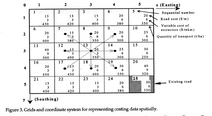
A costing network for extraction, transport or road construction can be formulated based on the grid system used for representing spatial data (Figure 3). Nodes are defined by grid cell centres and links are connections between adjacent nodes (cells) (Figure 3); each node having the same value as that of the grid cell. A node may have a maximum of eight links. For example, node 13 has eight links to its neighbour nodes (7, 8, 9, 12, 14, 17, 18, and 19), while node 1 has only three links to nodes 2, 6, and 7, as shown in Figure 3.
A link between two nodes for this type of costing network is associated with values of two kinds: (1) the distance; (2) the cost that is equal to the distance times the average cost per unit of distance. Figures 4 and 5 show the computed link values from each of the nodes to its neighbouring nodes for costs of road construction and wood extraction, respectively.
The networks shown in Figures 4 and 5 are ready for determining the shortest routes for road construction and wood extraction from a point to another. Shortest path models can be used for determining the minimum cost routes for extraction, transport and road construction, respectively. Djikstra's Algorithm [2] was found to be very efficient for determining the shortest paths from a source node to a destination node or from a source node to all other nodes within the given network. Figure 6 is an example of the shortest routes output.

To minimise computations during the running of the road locating procedure, the shortest routes of extraction, transport and road construction between every two nodes within the given network are determined beforehand using Dijkstra's Algorithm. If the Dijkstra's Algorithm is applied once to a node, the shortest paths from this source node to all other nodes within the network can be determined. If Dijkstra's Algorithm is applied n times, where n is the number of nodes in the network, to every node within the network, the shortest paths from any node within the network to all other nodes are determined. A detailed description of this n-application Dijkstra's algorithm is given in an earlier report by the author [16]. The outputs from the shortest path model are stored in Journal of Forest Engineering the tables of costs and paths from source nodes to destination nodes.
A Heuristic Road Locating Algorithm
The essential component of the network extension tools subsystem is the heuristic algorithm. The aim of the heuristic procedure was to determine the optimal location for a forest road network. It is applied after the costing and routing subsystem has established the necessary spatial database and the shortest routes for road construction, wood extraction and transport.


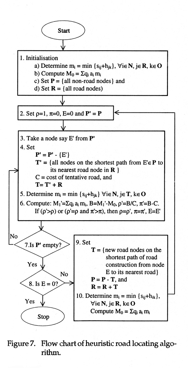
The heuristic method of solution, in general, relies on experience, inductive reasoning, or intuitive and empirical rules that have the potential to determine an improved solution relative to the current one. The heuristic algorithm is actually a repetitive search procedure (Figure 7) that extends the road network from one route segment to another in a way that most improves the model objective (maximization of net benefit or ratio of benefit to cost) at each step. When the road network can not be improved by the addition of a further route segment, the model objective is satisfied and the best solution possible for the road network location has been attained.
The road locating procedure extends the road network by the most feasible route at every step of the searching process. A route is feasible if building a road along it reduces the total cost of road construction, wood extraction and transport. In other words, a road route is economically feasible if the reduction in transport cost is greater than the cost of the road network extension. If the road network density in terms of road length per unit area (m/ha) is low, the appropriate extension of the road network may reduce the total cost. If there is at least one feasible route, the road network will be extended.
The best feasible route can be determined by applying one of the following two criteria.
(1) Maximising net benefit. The benefit is defined as the reduction in the amount of the extraction and transport costs. The cost of road construction is regarded as the cost incurred when gaining the benefit. The best route is the one that produces the highest net benefit. Any route under consideration must be feasible (benefit is greater than cost or the net benefit is greater than zero). This method can be expressed as follows (Symbols refer to Figure 8).
Maximise π = B - C on the left of Figure 10 is better than that on the right.
subject to
B - C > 0
(2) Maximising the ratio of benefit to cost. The feasible route that produces the highest ratio of benefit to cost is considered as the best. A route is feasible if the ratio of benefit to cost is greater than one. This method can be expressed as follows.
Maximise ρ = B/C
subject to
B/C>1

The experience gained from the use of these two criteria during this study showed that there was little difference in the result when locating a forest road network. A longer route tends to be selected using the net benefit criterion while the ratio criterion tends to select a shorter one. Generally, the longer road has a larger area of influence and hence creates greater a benefit in comparison with the shorter road. However, ratio of benefit to cost may be higher for a shorter route than a longer one because the longer route may sometimes contain an expensive route segment. To avoid the inclusion of an expensive route segment, the ratio criterion should be used. The net benefit criterion can be used to decide between two routes with equal ratio of benefit to cost. If this still results in a tie, the solution can be chosen arbitrarily.
The searching procedure includes the following steps.
(1) Assume a road route from one of the non-road nodes to its nearest road node.
(2) Compute the ratio of benefit to cost for the assumed road route.
(3) Repeat the above two steps until all non-road nodes are checked.
(4) Select the road route with the highest ratio of benefit to cost as the best feasible road route.
(5) Update the road network to include the best feasible road route.
(6) Repeat the above steps until no feasible road route exists.
This searching procedure is illustrated in Figure 7 and the symbols used are defined in Figure 8. Details of the heuristic algorithm were described in [16]. Applying this algorithm to the data shown in Figure 3, we obtained the solution for an optimum road network as shown in Figure 9. Outputs of costs and benefits from each step of the search are given in Table 1.
The cost of road construction is the sum of link values on the new road route as shown in Figure 9, which is $26 242.64. The benefit is the difference between wood movement costs before and after the new road is added into the area, which is $97 249.90. They are computed as follows. (1) Before the new road is added, there is only one road node (node 25) in the area as shown in Figure 4. Wood could be extracted from any node to the single road node only along the shortest path. The total cost of wood movement before new road is $904 434.40, including an extraction cost of $496 114.40 and a transport cost of $408 320.00. (2) After the new road is added as shown in Figure 9, the average extraction distance is shorter and hence extraction cost is lower, but transport distance is extended and transport cost is increased. The total cost of wood movement before the new road was $807 184.50, including an extraction cost of $395 697.40 and a transport cost of $411 487.10.
OPTIMISING ROAD NETWORK LOCATION
Road Network Location Assisted by Costing
and Routing Subsystem

Although the CARS subsystem presented above does not determine an optimal location for a forest road network, it facilitates the computation of costs and benefits for any given road route(s). Traditionally, the road planning manager begins identifying alternatives for road network location and then evaluates each alternative so that the best alternative can be selected from the identified alternatives (Figure 1). Costs and benefits can be computed through the CARS subsystem if the road planning manager inputs the alternatives into the system. Take the road planning project from previous study [16] as an example. Two alternatives for location of a forest road network were produced by a road planning manager as shown in Figure 10. These two alternatives can be added to the existing road network and then costs and benefits were computed, as shown in Table 2, using the CARS subsystem. Although it was possible in the previous version [16], it was difficult to generate road routes over the spatial database as the section of network modules was programmed on a mainframe computer. Now, by integrating the spatial database and network routing modules on a microcomputer the user interface and road route selection process is much easier. Once the costs and benefits for each of the alternative road network locations are known, it is not difficult to select the one that best achieves the planning objectives. Table 2 shows that the alternative on the left of Figure 10 is better than that on the right. The route on the left produces a higher net benefit
Table 1. Results at each search (iteration) of the heuristic road locating procedure.
|
Iteration
|
Road nodes extended
|
Road length
|
Cost, $
|
Benefit $
|
Ratio
|
Net $
|
||||
|
From
|
Via
|
To
|
m
|
Road
|
Extraction
|
Transport
|
||||
|
0
|
-
|
-
|
-
|
0.00
|
0.00
|
496114.40
|
408320.00
|
-
|
-
|
-
|
|
1
|
25
|
24
|
23
|
400.00
|
8500.00
|
442346.10
|
409571.20
|
52517.13
|
6.18
|
44017.13
|
|
2
|
23
|
-
|
17
|
282.00
|
4242.64
|
421808.40
|
410344.40
|
19764.56
|
4.66
|
15521.92
|
|
3
|
17
|
-
|
12
|
200.00
|
3000.00
|
411984.40
|
410877.40
|
9350.87
|
3.12
|
6350.87
|
|
4
|
12
|
-
|
7
|
200.00
|
3000.00
|
405400.80
|
411066.30
|
6334.75
|
2.11
|
3334.75
|
|
5
|
7
|
8
|
9
|
400.00
|
7500.00
|
395697.40
|
411487.10
|
9282.63
|
1.24
|
1782.63
|
| Total at optimum solution |
1482.84
|
26242.64
|
395697.40
|
411487.10
|
97249.94
|
1.24
|
71007.30
|
|||

($57 505.20) than the one on the right ($35 948.23). The optimal solution can be obtained by a process of interaction between the road planning manager and the CARS system. In the previous section, it was demonstrated that the heuristic algorithm determines an approximate optimum solution for locating forest roads. The heuristic algorithm was further tested on a microcomputer using data from a practical road planning project adapted from previous study [16], as described in the next section.
OPTIMUM ROAD NETWORK LOCATION
USING THE HEURISTIC PROCEDURE
As mentioned earlier, the road locating procedure was written in MS Visual Basic and applied under a MS Windows 95 environment. In order to test the capability of the system, data from a practical forest road planning project in North Finland were adapted. Most data for the road network planning were estimated and recorded according to compartments, within which forest stands and environmental conditions were considered to be homogeneous. Cost data were obtained from many sources including the forest management planning database, local forest inventory and survey, and estimations made by road planning experts. The study area was coded into a network of 557 nodes (grid cells), each having an area of 1 ha. 12 overlays of data were needed in order to consider all the factors for computing the costs of road, extraction, and transport. The project data were detailed in [16].
The results associated with the optimal road location determined using the heuristic road locating procedure on a microcomputer are listed in Table 3 and the optimal road network location is plotted over the data overlay for the allowable cut as shown in Figure 11. It should be mentioned that the allowable cut is only one of the 12 overlays used for computing the costs of extraction and transport. It is used to represent the area as it contains some information related to the boundaries of compartment. Details referred to [16].
When the road locating procedure was run on an IBM compatible Pentium 100 MHz microcomputer with sufficient memory and disk storage, total computation time was 34 minutes. This is 6 minutes shorter than a similar run described in the previous study [16]. That is to say that the microcomputer used for testing this program is similar to (may be better than) the mainframe computer used previously [16]. Of course, the performance of mainframe computers is faster today than then. However, it is much more convenient to run this program on a microcomputer rather than on a mainframe computer. It may be possible to use this method in actual field situations when planning forest road networks.
Table 2. Comparison of the two alternatives for a road network location shown in Figure 10.
|
Variables
|
Unit
|
Left
|
Right
|
| Total area |
ha
|
557.00
|
557.00
|
| Exist road length |
m
|
3197.06
|
3197.06
|
| New road length |
m
|
3514.21
|
3931.37
|
| Optimum road density |
m/ha
|
9.18
|
9.93
|
| Cost of new road |
$
|
41499.17
|
61469.57
|
| Cost of extraction |
$
|
120450.27
|
119936.17
|
| Cost of transport |
$
|
214911.76
|
212188.34
|
| Benefit of new road |
$
|
99004.37
|
97417.80
|
| Net benefit |
$
|
57505.20
|
35948.23
|
| Ratio of benefit to cost |
2.39
|
1.58
|
Table 3. Quantities computed for the optimum road location shown in Figure 11.
|
Variables
|
Unit
|
Value
|
| Total area |
ha
|
557.00
|
| Exist road length |
m
|
3197.06
|
| New road length |
m
|
3631.37
|
| Optimum road density |
m/ha
|
9.39
|
| Cost of new road |
$
|
42866.00
|
| Cost of extraction |
$
|
117076.80
|
| Cost of transport |
$
|
214861.60
|
| Benefit of new road |
$
|
102797.90
|
| Net benefit |
$
|
59931.90
|
| Ratio of benefit to cost |
2.40
|
Remarks on Computation
Variation in three parameters within the method will result in changes in the location solutions for the road network or changes in the computation time.
(1) The length of road extension at each search. The computation time is shortened if the length of road extension is set to a limit such as a dimension of the grid cell size (ie. 150 m to cover a diagonal distance of a cell of 1 ha area). For this reason, where there is a need to adjust computation time to take account of the ability of the microcomputer, it should always be done by varying the length of road extension. This will also change the location of the road network. For the selected study area, a length of 150 m was tested, using both the current revised system and the one from the previous study. It was found to be the best length of road extension when considering both computation time and optimum road network location.
(2) Maximum road influence area to be handled. Road influence area is the area around the road where
all transport from the area is made through that road only. When the road influence area is great, a large array of grid data must be processed to produce the shortest paths, which requires more computer memory and time. Since computer memory space is always limited, the road influence area must not be too large. On the other hand, when the road influence area is small, only a small reduction in extraction cost will result from building the road. Since the reduction in extraction cost is defined as the benefit from building the road, a small area of influence for a potential road produces a small benefit and may make the road infeasible. The road influence area is directly proportional to extraction distance. An extraction distance of 900 - 1 500 m proved to be the best for obtaining an optimum road network with a relatively low requirement for computing time and memory space for the selected study area.
(3) The resolution of grid system used. The resolution can be described by the size of the grid cell. The level of resolution in coding a network for road location is important in terms of reducing computation and maintaining accuracy.
The size of a cell in the grid is chosen to avoid two extremes:
(1) Too small a cell size may produce too many cells, and hence nodes for the costing network. Computation for a network with an excessive number of nodes may exceed the available capacity of the computer.
(2) Too large a cell size may produce too low an accuracy, which may not be acceptable to the end user. It is particularly difficult to define a road network when at the end of the road locating process almost every node in the network is selected as containing a road. The maximum size for a grid cell should not permit road cells to take up more than 50% of the total number of cells in the area; otherwise, spatial representation of such a road network will not be effective [7].
The appropriate size of the grid cells can be estimated by the following expression:

where
lc = side length of the grid cell, m
A = total area, ha
nmax = maximum number of grid cells that can be handled with the computer's capacity
dmax = maximum road network density, m/ha
Take the microcomputer system used for testing this program as an example. Assuming that the computation time is restricted to a maximum of 1 hour, nmax is about 1000 (estimated from a test of the current computer system). Suppose we have an area of 1000 ha, the minimum side length of a grid cell is then:

If the maximum road network density is about 12.5 m/ha (this can be estimated by finding out the optimal road network density), the maximum side length of a grid cell is:

lmax = 5000/12.5 = 400 m
Any size for a grid cell side length between 100 m and 400 m can produce satisfactory results.
To test and demonstrate the computation capability of the program on the microcomputer, the resolution for coding the study area and data was changed to a cell size of 50 m by 50 m, ie. an area of 0.25 ha. The study area was then represented by a network of 2196 nodes in an area of 549 ha. The total area was decreased to reduce the computation time without influencing the testing or the results. The final network result is shown in Figure 12. This is similar to that in Figure 11. The computation time was 26 hours 7 minutes. Based on the experience of this application, it is suggested that a network about 1000 nodes or less be used in order to keep the computation time below 1 hour. If the grid cell is set at 1 ha, a network of 1000 nodes will cover 1000 ha and this will meet the needs for most harvesting planning.
CONCLUSIONS


This paper presents a microcomputer-based spatial and heuristic procedure that was improved from a previous study [16] to provide two types of road locating aids for a forest road planning manager. Firstly, the CARS subsystem was improved to assist cost and benefit analysis for a given location of a forest road network. Using the techniques of Geographic Information Systems (GIS) and Operations Research (OR), the procedure enables both the spatial variations of forest stands and terrain which influence the optimum location of a forest road network to be considered. Integration of spatial database and network routing modules in a microcomputer improves the user interface and makes it easier for road planning manager to generate and assess (compute costs and benefits) alternatives of road network location, and hence select the optimal location. Secondly, the NETS subsystem contains a heuristic road locating procedure capable of locating forest roads within a given area, which minimises the total costs and impacts of road construction, extraction, and transport. A recent development to this subsystem was a road locating procedure using dynamic programming, which will be presented in another paper.
Acknowledgement
I would like to express my sincere thanks to Drs. Ryde James and Jeff Glaubitz, and two anonymous referees who provided valuable comments on improving the manuscript.
EDITOR'S NOTE: Australian $1.00 = US $0.66 (approximately).
References
[1] Dahlin, B and Sallnas, O. 1992. Designing a forest road network using the simulated annealing algorithm. In: [11]. P. 36-41.
[2] Dijkstra, E.W. 1959. A note on two problems in connection with graphs. Nemerishe Mathematik I (1959): 269-271.
[3] Hitrect, V. and Dalbello, B. 1992. Computer-aided opening of forest stand by stand partition. In: [11]. P. 42-47.
[4] Larsson, G. 1959. Studies on forest road planning. Transportation of the Royal Institute of Technology 147. Stockholm. 136 p.
[5] Li, G., Wang, L. and Tang, D. 1992. Computer supported planning of roads for cable logging in southwest China. In: [11]. P. 48-52.
[6] Matthews, D.M. 1942. Cost control in the logging industry. McGraw-Hill Book Company, Inc., New York. 374 p.
[7] Nitami, T. and Kobayashi, H. 1992. Systemising of forest-road planning work. In: Whyte, A.G.D. and Allen, J.C. (eds). A compendium of papers to be presented at IUFRO S3.04.01 Conference, Christchurch, 27-3`, January, 1992, New Zealand School of Forestry, University of Canterbury. p. 155-163.
[8] Peters, P.A. 1978. Spacing of roads and landings to minimise timber harvest cost. J. For. Sci. 24 (2):209-217.
[9] Pulkki, R. 1996. Water crossing versus transport cost: a network analysis case study. Journal of Forest Engineering 7(2): 59-64.
[10] von Segebaden, G. 1964. Studies of cross-country transportation distances and road net extension. Studia Forestalia Suecica 18. Stockholm. 69 p.
[11] Sessions, J. (editor) 1992a. Proceedings of Computer Supported Planning of Roads and Harvesting Workshop. IUFRO S3.05 and S3.06. and University of Munich, Feldafing, Germany. 316 pp.
[12] Sessions, J. (editor) 1992b. Using network analysis for road and harvest planning. In: [11]. P. 26-35.
[13] Sever, S. and Knezevic, I. 1992. Computer-aided determination of optimal forest road density in mountainous areas. In: [11]. P. 13-25.
[14] Shiba, M. 1992. Optimization of road layout in opening up of forests. In: [11]. P. 1-12.
[15] Sundberg, U. and Silversides, C.R. 1988. Operational efficiency in Forestry. Vol. 1: Analysis. Kluwer Academic Publishers. 219 p.
[16] Tan, J. 1992. Planning a forest road network by a spatial data handling-network routing system. Acta Forestalia Fennica 227. The Society of Forestry in Finland - The Finnish Forest Research Institute. Helsinki.
[17] Tucek, J. and Pacola, E. 1999. Algorithms for skidding distance modelling on a raster digital terrain model. Journal of Forest Engineering 10(1): 67-79.
[18] Wang, L. 1992. Computing optimal combination of seasonal and all season roads for harvesting operations in China. In: [11]. P. 53-56.