
Display large image of Figure 1
Vol. 11 No. 2 July 2000
J. Tan
Department of Forestry
The Australian National University
Canberra, Australia
ABSTRACT
The optimum solution of locating a forest road network in a given forest area is still difficult to determine due to the complexity and the nature of the problem. Heuristic solutions are estimations of the optimum location but not the optimum one. This paper presents a dynamic programming procedure, integrated with microcomputer-based spatial database and transport network models, which can be used to assist foresters in determining the optimum location for a forest road. This method contributes to the optimum location of an entire road network serving a forest area.
Keywords: Forest roads, location, planning, dynamic programming, and networks.
The author is a Lecturer with the Department of Forestry.
INTRODUCTION
Recent research has resulted in more and more applications of computer technology, which facilitates the solving of forest road location problems [1, 4,6, 8, 9]. The usefulness of these applications is that they enable the consideration of spatial variation of forest environments and resources by applying techniques of geographic information systems (GIS) and operations research (OR). Finding the optimum solution for locating a forest road network for a given forest area is still not possible due to the complexity and the nature of the problem. Many of the heuristic methods used in locating a forest road network are estimations of the optimum solutions [8, 9]. This study attempts to determine the optimum solution for locating a forest road applying dynamic programming.
Dynamic programming (DP) was designed primarily to improve the computational efficiency of solving certain mathematical programming problems by decomposing them into smaller, and hence computationally simpler, sub-problems [3,7]. Unlike the heuristic programming which determines an optimum solution just for each sub-problem but where the overall optimum solution is not obtained, dynamic programming determines a solution that is
optimum after the last sub-problem is solved. Many of optimum solutions for road location using dynamic programming depend very much on the starting and end points, or partitioned basic units such as compartments [5] or grid cells [2] and the methods of cost computation. The DP procedure presented in this paper has greater flexibility in dealing with boundary problems.
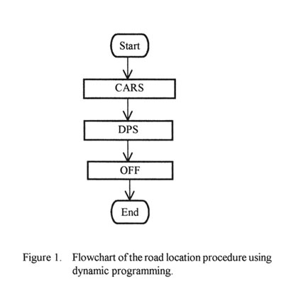
The road locating procedure using DP (dynamic programming) includes two main modules: costing and routing sub-system (CARS) for road construction, extraction, and transport, and dynamic programming sub-system (DPS) for optimum location of one road as shown in Figure 1.
Figure 1: Flowchart of the road location procedure using dynamic programming.
Display large image of Figure 1
The dynamic programming procedure is applied to solving the road location problem after the spatial database and shortest path models have been established. The spatial database and the shortest path models for costing and routing of road construction, extraction and transportation are part of CARS (Figure 1) and were described in [8,9b]. This paper will present details of the dynamic programming sub-system (DPS in Figure 1) and results of testing the procedure using a practical road location project. Its capability and limitations in application comparing with heuristics and other DP solutions will be also discussed.
The method for optimising forest road location in this study focuses on internal forest roads. Internal forest roads are located within a forest area and they serve mainly to provide access for forest operations (forest stand establishment, stand improvement, stand protection, and logging). Consideration of roads built for uses such as fire isolation in addition to transportation is beyond the scope of this study. This paper does not cover the study on data collection. Data may come from many sources such as forest management documents, geographic information systems (GIS) and global positioning systems (GPS) applied to forest management, expert knowledge, reconnaissance in the field and so on. Road engineering design and field construction are not dealt with in this study.
Formulation of Dynamic programming (DP) model
Dynamic Programming Model Elements
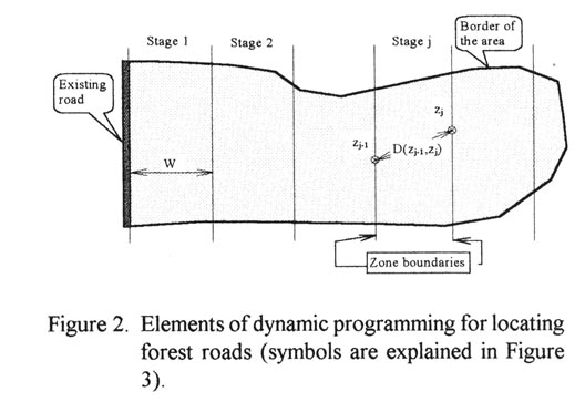
To build the dynamic programming model, the road planning area given is divided into zones as shown in Figure 2. Zones are separated by zone division boundaries. The boundaries are supposed to be parallel (equidistant) to the road. Theoretically, all points on the same boundary of a zone have a constant distance to the road. The distance between any two boundaries is the same, ie, the zones are of the same width. The boundaries are numbered with the road route as boundary 0, the boundary being the nearest to the road route as boundary 1, and the boundary being the furthest away from the road route as boundary nz. Here, nz is the total number of zones.
Figure 2: Elements of dynamic programming for locating forest roads (symbols are explained in Figure 3).
Display large image of Figure 2
After dividing the area into equidistant zones, the elements of dynamic programming model [7] are defined below.
1. Stage j represents zone j.
2. State zj-1 at stage j is the node at the end boundary of zone j-1, which is also the node at the start boundary of the zone j.
3. Alternative zj-1 for zj at stage j is the node at the end boundary of zone j-1. Route (zj-1, zj) is the alternative route linking node zj at the end boundary of zone j to node zj-1 at the end boundary of proceeding zone j-1.
Let fj(zj) be the maximum net benefit accumulated from stages 1, 2, …, j given zj is the node at the end boundary of stage j. The recursive equations are thus given as follows (Figure 2):
(1) f0(z0) = 0
(2) fj(zj)
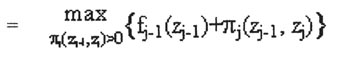
Where
zj-1, zj = nodes at the end boundary of zones j-1 and j
pj(zj-1, zj) = net benefit gained by building a road between nodes zj-1 and zj
The feasible condition in selecting a road route is
pj(zj-1, zj)>0 that is the restriction built in the equations above.
DP Model for Locating Forest Roads
The dynamic model formulated in the previous section can be implemented by Visual Basic on a microcomputer. For ease of computer programming and for the convenience of demonstration, the dynamic programming equations are expressed as follows:
(3) f0(z0) = 0
(4) fj(zj)
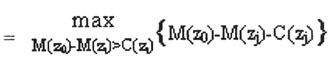
Where
M(zj-1), M(zj) = minimum total cost of timber
extrac-tion and transport from existing road to nodes
zj-1 and zj, respectively
C(zj) = minimum total cost of road from existing road to node zj
C(zj) 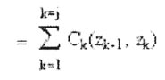
Ck(zk-1, zk) = cost of building a road between nodes zk-1 and zk at stage k.
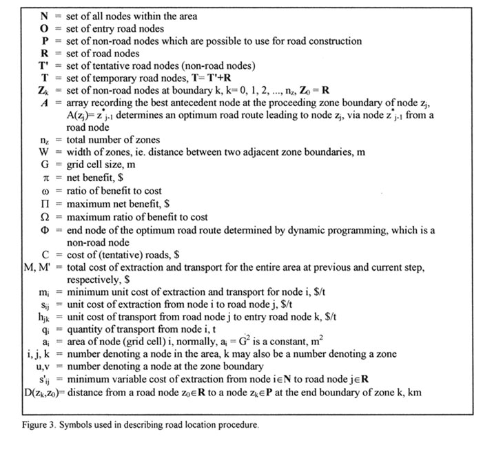
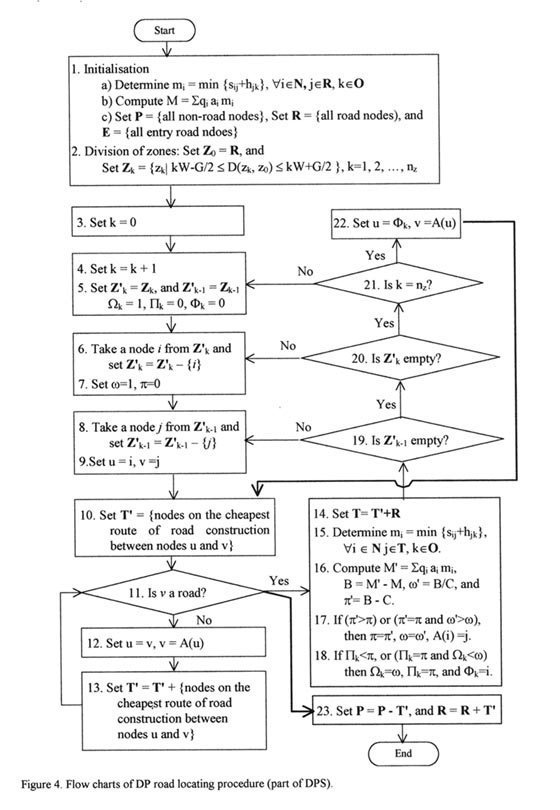
The difference between M(z0) and M(zj) is the total benefit. Therefore, the computed quantity in the second equation is the total net benefit. Other symbols used in describing the dynamic programming road locating procedure are listed in Figure 3. The flow chart of the procedure is shown in Figure 4.
Figure 3: Symbols used in describing road location procedure.
Display large image of Figure 3
Principally, the road locating procedure by DP is to determine array A(zj) which contains nodes that are antecedent to node zj. A(zj) can be described as follows:
· A(zj) is a node at the end boundary of zone j-1;
· A route connecting a road node via A(zj) produces the best road route leading to zj.
· Nodes on the optimum road route leading to zj can be retrieved by the process: zj, A(zj), A(A(zj)), …, until a road node is reached (steps 15 to 18, Figure 4.
If A(zjj) is determined for j=1, 2, …, nz, the optimum road routes leading to all nodes at the farthest boundary are determined. The node zn at the last boundary that produces the highest objective value is recorded as F. If F is equal to 0, there is no optimum road route leading to the last boundary. If F is not equal to its original value (ie. 0), the optimum solution is achieved. Further optimisation programming needs to be done as discussed later in next section about the optimisation of the road endings.
OPTIMUM LOCATION OF A FOREST ROAD USING DYNAMIC PROGRAMMING
Implementation of DP Road Locating Procedure with a Practical Road Planning Project
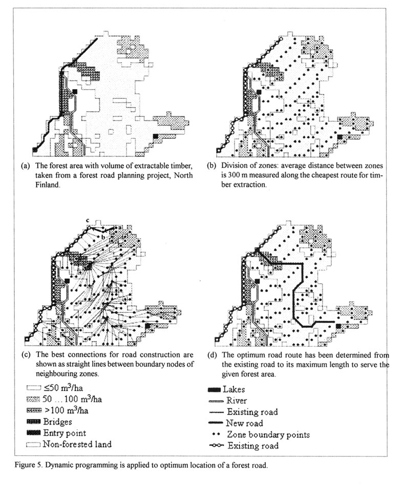
Data from a practical forest road-planning project in North Finland used in previous studies [8,9b] were adapted to test the applicability of DP procedures. The digitised area with volume of extractable timber is shown in Figure 5a. Twelve data overlays were created in order to determine the costs of extraction, transport and road construction. The shortest paths for extraction, transport and road construction are determined before applying the dynamic programming method. Details related to the data overlays and the shortest paths are given in the literature [8]. This section will focus on the application of DP procedures.
Figure 4: Flow charts of DP road locating prodecure (part of DPS).
Display large image of Figure 4
Dynamic programming solves the road location problems by multiple stages. The stages are defined by dividing the whole area into zones of equal width. Figure 5b shows the boundary nodes of the zones, where the average distance between boundaries of neighbouring zones is 300 m. This is a parameter which can be changed according to the users' requirement. The nodes on a boundary have the same distance to the existing road. The distances are measured along the cheapest route for timber extraction.
Once the boundaries for the zones or stages are defined, the dynamic programming equations shown in expressions 3 and 4 can be applied to determine the best route for road construction from the previous boundary to current one for every node at the current zone boundary. The best routes for road construction between boundary nodes of neighbour zones are determined in the order that begins the boundary nearest to the existing road and ends with the boundary farthest from the existing road. Figure 5c shows the best connections between nodes of neighbour zones determined by DP procedure (Figure 4).
From the results shown in Figure 5c, the best route for road construction from the existing road to any node at the boundary of a zone can be traced backwards. For instance, the best road route to point a is a®b®c, where c is a node of existing road. For a given problem, the number of best road routes are many. The best route linking a non-road node to the existing road network may or may not be feasible. However, the optimum road route must be feasible and produce the maximum net benefit such as the road route shown in Figure 5d.
Feasible Ending of a Road
The optimum road determined by the procedure described above will always be economically feasible. However, one or more parts of the road extended at a step of the procedure may not be feasible although the entire road route is feasible and optimum. For example, part of the road may require a culvert or bridge for crossing a stream. Such a road structure is usually very expensive and may result in an unfeasible solution for extending the road network to the next zone. However, when the entire road is extended over a longer distance the solution may be feasible and can be optimum. This case is covered in the process of road locating using dynamic programming. This is an important distinction between heuristic and dynamic programming methods. When heuristic methods are used, all sections of road extension must be feasible extensions.
It is possible that the unfeasible section of the road may occur at the last zone. In this case, the last section will be excluded. The unfeasible ending of a road route is checked by a subroutine of the program. The optimum road route shown in Figure 5d has been processed using this subroutine. It is optimum and does not contain any unfeasible ending.
Division of Zone Boundaries
The zones defining the stage of dynamic programming can be varied using different distances between boundaries. The distance between zones can be measured as the beeline distance or as the shortest distance for extraction. From experience gained while testing the method described in this study, it was found that the beeline distance might result in zone boundaries perpendicular to the road if the area is divided by geographic feature, for example by a river. Then distance between the zones may be too long and hence the capability of optimisation by DP procedure is reduced. Therefore, the minimum cost paths are used, which show the high cost positions such as those places crossing over a river.
The distance between zones measured at the minimum cost paths can be varied depending on the capability of the computer systems and size of the grid cell. The minimum distance between zones is the size of the grid cells. The maximum distance between zones is limited by the width of the neighbourhood region at a node if it is used. More explanations of the neighbourhood region are given in the texts for Figure 9 and details refer to literature [8,. In reality, the number of possible connections will be reduced to only one or two if the distance between zones is set to the maximum value, which is the width of the neighbourhood region. Then there is no great need to carry out an optimisation procedure using computers because one or two solutions can be easily determined manually. To avoid the situation where the feasible solutions are too few, the distance between zones should be much shorter than the width of the neighbourhood region. It was found that very satisfactory results are produced when the distance between zones was set to be one third of the neighbourhood region width or less.
When testing the DP procedure using the data shown in Figures 5a to 5d, the distance between the zones was varied from 100 to 600 metres. It was found that a distance of 300 metres between the zones produced the best result when determining the location of a forest road as shown in Figure 5d without excessive computation time.
Figure 5: Dynamic programming is applied to optimum location of a forest road.
Display large image of Figure 5
To maximise the objective value, the default for the distance between zones was set to be 300 metres. The DP procedure determines the best connections between nodes of two neighbour zones by this zone width from the existing road to the most distant point of the given area. The route that produces the maximum objective values is selected and end of the road is evaluated and optimised as discussed earlier.
Optimisation Objectives
Similar to the heuristic programming method described in the previous studies [8,9b], either net benefit or ratio of benefit to cost can be used as the road location criterion or objective. However, unlike heuristic programming that determines an approximate optimum solution, the dynamic programming method can determine the optimum solution when the last stage is finished. Our desired objective is to maximise the net benefit. Therefore the net benefit is used as the objective value. When the last stage is completed, the dynamic programming solution will be optimum for the entire area within which the road, which gives the maximum net benefit, is located.
Comparison of Dynamic Programming with Heuristic Programming
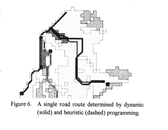
Locations of a single and longest road for the given forest area are shown in Figure 6. While dynamic programming method can be used to determine an optimum solution for the location of a forest road, computation time may be long in comparison with heuristic programming. However, although the heuristic programming method [8] is faster, it determines only an approximation to the optimum solution as shown in Table 1.
Figure 6: A single road route determined by dynamic (solid) and heuristic (dashed) programming.
Display large image of Figure 6
LOCATION OF A FOREST ROAD NETWORK
Location of Multiple Roads
Although the road locating procedure using DP will determine a road route that is optimum for connecting a remote node to the current road network, the optimum solution is just one road route. As one road route may not be enough to cover the entire area, the whole road network may not be optimum. Increase in road network density may still reduce the total cost of extraction, transport and road construction.
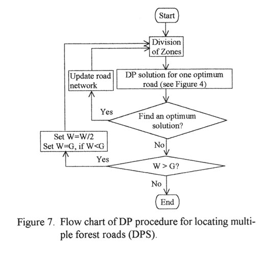
The road network should be extended after the first optimum solution for a road is determined. Other routes can be located by the same procedure as shown in Figure 4. The procedure can be repeated until no more extension is feasible. This process is similar to the way the network is developed using heuristic programming and can be described using flowchart as shown in Figure 7.
Table 1. Comparison of computations for locating a single forest road using dynamic and heuristic programming on a Pentium 100 MHz microcomputer.
| Computations at optimum | Dynamic programming | Heuristic programming |
| Calculated max. net benefit ($) | 55148 | 54147 |
| Extended road cost ($) | 120098 | 106749 |
| Extended road length (metres) | 6628 | 6204 |
| Computation times (minutes) | 333 | 12 |
Once an optimum road is added into the current road network, the area is divided again into new zones. Another set of routes will be evaluated and an optimum location will be determined. The zone division and optimum solution processes can be repeated until no further optimum solution can be determined. Then the zone width should be halved if the zone width is greater than grid cell size. However, the minimum zone width must be greater than or at least equal to the grid cell size.
The procedure shown in Figure 7 therefore has the ability to locate more than one road. It ends when no further solutions for optimum location of new roads can be found. At this point, the road network will have reached its optimum density and the location of the road network is optimum. One such a solution is shown (thick solid route) in Figure 8.
Figure 7: Flow chart of DP procedure for locating multiple forest roads (DPS).
Display large image of Figure 7
Dynamic Programming vs. Heuristic Programming
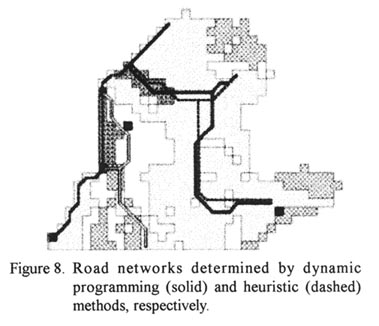
Two solutions for road location using dynamic programming and heuristic programming are compared as shown in Figure 8 and Table 2. Figure 8 demonstrates that the two methods give a difference in results for location of the road network. As mentioned earlier, dynamic programming method determines the optimum solution for a single road but it does not ensure an optimum for the location of more than one road. For two or more roads, the location of a forest road network is still an estimate of the optimum solution whether using dynamic programming or heuristic programming. Which one is better in achieving the best road network location depends on the nature of the given area. Factors like the shape of the area, wood volume and terrain conditions influence the results of road network location. However, it is very clear that the heuristic programming method is faster than dynamic programming method in general. Dynamic programming requires more computing resources than heuristic programming as shown in Table 2. The advantage of dynamic programming is that it ensures an optimum location for a single road. When more than one road need to be located both dynamic programming and heuristic programming methods can be applied but will result in different solutions. Forest road planning managers can select the one that best meets their requirements. One clear advantage of dynamic programming is that it is more capable in locating a road network past expensive areas if the overall solution is feasible. This is demonstrated in the next section.
Figure 8: Road networks determined by dynamic programming (solid) and heuristic (dashed) methods, respectively.
Display large image of Figure 8
Table 2. Computations for the location of road networks shown in Figure 8 using DP and heuristic methods on a Pentium 100 MHz microcomputer.
| Computations at optimum | Dynamic programming | Heuristic programming |
| Maximum net benefit ($) | 58397 | 62184 |
| Extended road cost ($) | 128548 | 128598 |
| Extended road length (m) | 6870 | 6828 |
| Computation times (minutes) | 488 | 19 |
Road Crossing Streams
As previously mentioned the DP method was better than heuristic methods for considering solutions beyond expensive sections of roads, such as river crossings. Heuristic programming methods developed in previous studies [8, 9b] are limited when considering the extension of the road over an expensive road section. For heuristic programming the neighbourhood region is used, particularly in microcomputer applications, to save memory space and computing time. However, the dynamic programming can continue to calculate the added benefit from areas that are located away from the existing road structure. This is the distinct advantage of DP over heuristic methods.
Dynamic programming methods result in an optimum road location over difficult terrain such as a river even if the neighbourhood region is limited. The process of heuristic programming may stop if using a neighbourhood region and encountering difficult terrain such as a river. The advantage of being able to include patches of difficult terrain implies that dynamic programming may be applied to locate a forest road for a large area; using the technique of neighbourhood region.
The neighbourhood of a node consists of the surrounding (adjacent) nodes: the node itself along with the four immediate non-diagonal and four diagonal nodes. The "neighbourhood region" of a node is an extension of the neighbourhood concept to include all nodes that are located within a predefined distance surrounding the given node. The technique of neighbourhood region is used to confine the optimisation procedure to search only within a region that is smaller, in terms of number of nodes, than the entire planning area. It is used, therefore, to reduce the consumption of computer resources. The concept of "neighbourhood region" is explained in detail in previous publications [8, 9b].
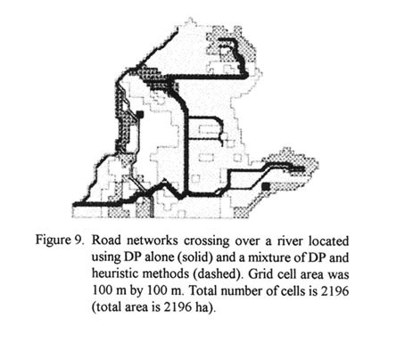
Figure 9 is the result of road location by dynamic programming when the original data were magnified to be almost four times the original size. Calculations for the road network location were based on an extraction distance of 900 meters which was modeled by considering a neighbourhood region of 9 cells around, that is 361 cells (a square block of 17 by 17 cells). The same data were used to test the heuristic programming method but in this case the method could not consider extending the road over the river due to the neighbourhood region being too small. It is clear that dynamic programming has better capacity than heuristic programming to consider difficult terrain such as a river.
Figure 9: Road networks crossing over a river located using DP alone (solid) and a mixture of DP and heuristic methods (dashed). Grid cell area was 100 m by 100 m. Total number of cells is 2196 (total area is 2196 ha).
Display large image of Figure 9
A major disadvantage to running this dynamic programming procedure to locate a road network for such a large area is the computation time. The calculations took 141 hours to complete (Table 3). A modification of dynamic procedure was carried out so that once the road network was extended over the river the heuristic programming was used. This modification reduced the computation time to 7 hours (Table 3). The result obtained by this modification is similar to that using dynamic programming alone.
CONCLUSIONS
This paper presents a dynamic programming procedure that can be used for determining the optimum location of a forest road. The procedure was tested using data from a practical road planning project. Results of testing dynamic programming were also compared with those using heuristic programming [8,9b]. It was found that dynamic programming determined the optimum solution for location of a forest road, unlike an estimation of the optimum location for a road by the heuristic programming method. However, the computation time by the dynamic programming was longer than that by the heuristic programming.
Table 3. Computations for location of roads crossing over a river using DP or combination of DP and heuristic programming on a Pentium 100 MHz microcomputer.
| Computations at optimum | Dynamic programming alone | Combined use of DP and heuristic methods |
| Calculated max. net benefit ($) | 247223 | 253824 |
| Extended road cost ($) | 628031 | 636312 |
| Extended road length (metres) | 3320 | 23444 |
| Computation times (hours) | 141 | 7 |
When locating a road network where there is more than one road, the dynamic programming method does not determine an "optimum" solution. Its results are not better than the heuristic programming method. However, the dynamic programming method has the capacity to consider forest beyond difficult terrain such as a river when using the so-called neighbourhood region on microcomputers, while the heuristic programming method has limitations in doing so. It can be beneficial to combine dynamic programming and heuristic programming. The heuristic programming is used for its ability to provide results quicker when using microcomputers. Dynamic programming should be used to find an optimum solution if only one road is to be located. Dynamic programming can also be used for considering difficult terrain where expensive sections like river crossings limit the scope of heuristic methods.
ACKNOWLEDGEMENT
The author wishes to thank Dr. Ryde James and two anonymous referees for their comments on improving the manuscript.
AUTHOR CONTACT
Dr. Jimin Tan can be reached by e-mail at --
jimin.tan@anu.edu.au
REFERENCES
[1] Dean, D.J. 1997. Finding optimal routes for networks of harvest site access roads using GIS-based techniques. Canadian Journal of Forest Research 27:11-22.
[2] Douglas, R.A. and Henderson, B.S. 1987. Computer assisted forest road route location. In: Proceedings of the Council on Forest Engineering 10th annual meeting. High technology in Forest Engineering, 1987. Syracuse, New York. 201-214 p.
[3] Dykstra, D. P. 1984. Mathematical programming for natural resource management. McGraw-Hill Book Company, New York. 318 p.
[4] Nieuwenhuis, M. 1986. Development of a forest road location procedure as an integral part of a map based information system. University of Maine. 193 p.
[5] Sakai, T. 1984. Studies on planning method of forest roads network. In: Proceedings of IUFRO Symposium on Forest Management Planning and Managerial Economics at University of Tokyo. 363-370 p..
[6] Sessions, J. (editor) 1992. Proceedings of Computer Supported Planning of Roads and Harvesting Workshop. IUFRO S3.05 and S3.06. and University of Munich, Feldafing, Germany. 316 p.
[7] Taha, H.A. 1982. Operations research: an introduction. MacMillan Publishing Co. Inc. New York. 848 p.
[8] Tan, J. 1992. Planning a forest road network by a spatial data handling-network routing system. Acta Forestalia Finnica 227. 85 p.
[9] Tan, J. 1999. Locating forest roads by a spatial and heuristic procedure on microcomputers. Journal of Forest Engineering 10(2):91-100.