Geology and Wine 9: Regional Trace Element Fingerprinting of Canadian Wines
John D. GreenoughDepartment of Earth and Environmental Sciences, University of British Columbia -Okanagan, 3333 University Way, Kelowna, B.C., Canada, V1V 1V7
John.Greenough@ubc.ca
Leanne M. Mallory-Greenough
Department of Earth and Environmental Sciences, University of British Columbia -Okanagan, 3333 University Way, Kelowna, B.C., Canada, V1V 1V7
Brian J. Fryer
Department of Earth Sciences, University of Windsor, Windsor, Ontario, Canada, N9B 3P4
SUMMARY
New, and previously determined, trace-element analyses (20 elements) for 162 wines from five regions across Canada (Nova Scotia, Quebec, Ontario (Niagara and Pelee Island) and British Columbia (Okanagan and Vancouver Island) test the hypothesis that wines can be regionally "fingerprinted", using routine ICPMS analyses. Exploratory statistics show that wine trace-element composition is predominantly related to region of origin and wine colour. Compared to white wines (128 samples), red wines (34 samples) have higher Rb, Cs, Sr, Ba and M and lower Li, U and Th. This may be explained by extraction from grape skins (Rb, Cs, Sr, Ba, Mo) and adsorption onto grape skins (Li, U, Th) during fermentation of red wines, although other explanations (e.g., bisulfite addition) cannot be ruled out. Nearly all 20 trace elements are useful for creating discrimination diagrams that separate wines by region with considerable accuracy (>90%). The geochemical behavior of trace elements in all wines suggests that a common mechanism, the effect of climate on trace element solubility, affects trace-element concentration patterns. Further, regional average concentrations of most trace elements correlate strongly with Degree Days, indicating that more heat results in increased evaporation, which in turn increases water uptake, thus yielding higher trace-element concentrations in grapes. High Sr and Ba in Okanagan wines may be derived from alkaline soils in this semi-arid environment. Thus, terroir-related climate and soil differences lead to quantifiable trace-element fingerprints for Canadian wines by region.SUMMAIRE
Les résultats précédents et récents d'analyses d'éléments traces (20 éléments) sur 162 vins provenant de cinq régions du Canada (Nouvelle-Écosse, Québec, Ontario (Niagara et île Pelee) et de Colombie-Britannique (l'Okanagan et l'île de Vancouver) permettent de tester l'hypothèse selon laquelle il serait possible de caractériser régionalement les vins à partir d'analyses de routine de SM/PIHF. Une analyse exploratoire statistique des résultats montre que la composition en éléments traces est principalement reliée à la région d'origine des vins et à leur couleur. Comparés aux vins blancs (128 échantillons), les vins rouges (34 échantillons) ont des teneurs plus élevés en Rb, Cs, Sr, Ba et Mo, et moins élevés en Li, U et Th. Cela pourrait s'expliquer par un phénomène d'extraction à partir des peaux de raisin (Rb, Cs, Sr, Ba, Mo) et d'adsorption sur les peaux de raisin (Li, U, Th) durant la fermentation des vins rouges, bien qu'on ne puisse exclure d'autres explications telle (l'ajout de bisulfite par ex.). Presque chacun des 20 éléments traces contribue à la réalisation de diagrammes de différenciation qui permettent de départager les vins par région avec une grande précision (=90 %). Le comportement des éléments traces dans tous les vins permettent de penser qu'un mécanisme commun, soit l'effet du climat sur la solubilité des éléments traces, affecte les profils de concentration en éléments traces. De plus, les concentrations régionales moyennes de la plupart des éléments traces montrent qu'il existe une forte corrélation avec les degrésjours, ce qui indique qu'un surplus de chaleur amène un accroissement de l'évaporation, ce qui entraîne un accroissement de l'absorption d'eau, ce qui explique les plus fortes teneurs en éléments traces des vins. Les fortes teneurs en Sr et en Ba des vins de l'Okanagan pourraient s'expliquer par ses sols alcalins dans un environnement semi-aride. Et c'est ainsi que les facteurs climatiques et pédologiques permettent la caractériser de manière quantifiable les vins canadiens par région.
INTRODUCTION
1 In the early 1900s, the French began certifying the origin and authenticity of wines using the Appellation d'Origine Contrôlée (Johnson, 1991, p. 44). Underpinning this geographic certification was the idea that terroir (see Haynes, 1999, for a definition) determines the quality and character of wines. Today, quality wines from around the world bear labels testifying to where their grapes came from. In reality, it is difficult or impossible to quantitatively certify the origin of a bottle of wine. Given that individual wines can fetch thousands of dollars, and that organizations purchase millions of dollars-worth of wine assuming that the label actually reflects place-of-origin, the potential value of a simple method for verification is obvious.
2 During the mid-1990s, several studies indicated that trace elements in wines might be used to determine the origin of their grapes at vineyard and regional levels (Latorre et al., 1994; Stroh et al., 1994; Greenough et al., 1996, 1997). These studies left many unanswered questions. To what extent do processing methods affect the trace-element composition of wine? What happens to trace elements as wines age, and how much inter-year variability is there in wines from one vineyard or region? It is now known that these issues may confound the practical aspects of legal fingerprinting of wines, but the most important control on composition appears to be the geographic origin of the grapes (Taylor et al., 2002, 2003). Three other points have emerged:
- fingerprinting requires a multi-element dataset;
- multivariate statistical techniques are needed for data analysis; and
- one of the most promising analytical methods for trace-element fingerprinting of wines is Inductively Coupled Plasma – Mass Spectrometry (ICP-MS), which is inexpensive, routine and accurate.
3 Canada's small wine industry has an international reputation for producing fine wines, primarily from the Niagara and Okanagan regions of Ontario and British Columbia, respectively. Fledgling products from Nova Scotia, Quebec and Vancouver Island enjoy loyal local support. Taylor et al. (2003) showed that Okanagan and Niagara wines are distinguishable using ICP-MS trace-element data. The present study has two objectives:
- to determine if wines from the five Canadian wine-producing areas noted above can be "fingerprinted" with ICP-MS data; and
- to re-examine why red and white wines appear to have different trace-element compositions.
SAMPLES, GEOLOGY AND CLIMATE
4 Seventy-six bottles of wine, made from grapes derived from 35 vineyards, were purchased from 28 wineries in Nova Scotia (30 bottles; 12 vineyards; 5 wineries), Quebec (9; 5; 5), Ontario (Pelee Island, 2; 1; 1), the Okanagan Valley, British Columbia (16; 13; 13) and Vancouver Island, British Columbia (19; 4; 4). The emphasis was placed on obtaining wines made from grapes from a large number of geographically distinct vineyards representing the five main regions noted above (Fig. 1). Many Nova Scotia and Vancouver Island vineyards are represented by more than one wine sample. The 76 new samples of wine are augmented by data for 86 wines from the Niagara area of Ontario (36) and the Okanagan Valley (50) in the Taylor et al. (2003) study. Ice wines and late harvest wines were excluded because their production involves distinct processing and harvesting practices that affect trace-element concentrations. Altogether there are 34 red wines and 128 white wines in this study. Most wines were made from a single grape variety with > 42 varieties represented. Wines from Nova Scotia, Quebec and Vancouver Island are commonly made from hybrid grapes such as the popular Maréchal Foch (red) and Seyval Blanc (white). Okanagan and Niagara wines mostly use Vitis vinifera varietals with Chardonnay and Pinot Blanc (white wines), and Merlot and Pinot Noir (red wines) being important varieties; vintages range from 1992 to 2002.
5 Canadian vineyards are planted on a wide variety of soil types underlain by diverse bedrock geology (Table 1). Each wine producing area has distinctive climate characteristics reflected in annual precipitation, average temperature and number of Degree Days (= the cumulative amount of time above the threshold temperature of 10o C for each day of the growing season. For example, if the mean temperature of a day is 25o C, this would be 1 x 15 or 15 Degree Days; Table 1). This latter variable, in various forms, is used extensively in agriculture, and in the wine industry for identifying suitable locations for viticulture (Davis et al., 1984, p. 31). In addition to geo-chemical studies, relationships between geology and terroir for the Okanagan and Niagara regions are discussed in Haynes (2000), Fulton (2003), Grant et al. (2004), Greenough et al. (2004) and Bowen et al. (2005).
Figure 1. Map showing areas of Canadian wine production represented in this study.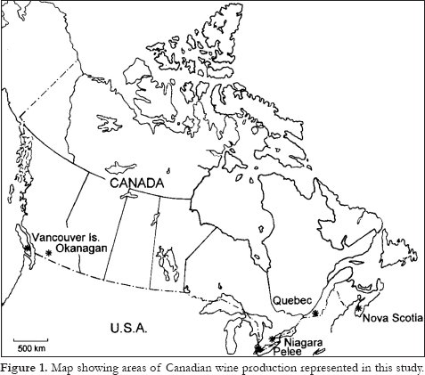
ANALYTICAL TECHNIQUES AND STATISTICAL METHODS
6 The 76 "new" wines were analyzed for 20 trace elements by using the ICP-MS at the University of Windsor. Wine samples were diluted 10:1 using high-purity 2% HNO3 that was spiked with internal standard elements (Be = 5, In = 0.5, Tl = 1 ppm) to correct for matrix effects and instrument drift during ICP-MS analysis. Elemental analysis was performed using a ThermoElemental X-7, ICP-MS unit coupled with a CETAC ASX 500 autosampler. ICP-MS calibration used 3 separate multi-element solutions (supplier = Inorganic Ventures Ltd.). Dilution blanks were measured from the internal standard spiked with 2% HNO3. Data reduction and correction for matrix effects, instrument drift, and molecular ion interferences used commercial spreadsheet software. Duplicate samples (one for every 20 wines) were collected during opening of the wines and treated as unknowns. Precision, based on the duplicates, is +/-1-2% except where close to the detection limit. Some of the 162 wine samples have Th (8 samples) or Ag (14 samples) below detection limits.
7 Data statistical analysis employed SYSTAT software. Multidimensional scaling (MDS; Wilkinson et al., 1992; Borg and Groenen, 1997, p. 1-14), an exploratory data analysis technique, was used to uncover natural patterns in the dataset. MDS yields "maps" of the distances between objects (trace-element compositions of wine samples in this study) based on a distance measure, in this case correlation coefficients. Two wines with identical concentrations of all trace elements would have a correlation coefficient of 1, whereas two wines with a perfect negative correlation would yield a correlation coefficient of -1. Using a matrix with all possible wine-versus-wine correlation coefficients, MDS yields diagrams in which chemically similar samples plot close together. Samples on opposite sides of an MDS diagram are most-different. MDS can also be used to compare the behaviour of elements by inverting the dataset (Fig. 2).
8 After determining the predominant relationships among samples using MDS (Fig. 3), discriminant analysis can help explain the origin of the data patterns and put them to use (Tabachnick and Fidell, 2001, p. 456-464; Rollinson, 1993, p. 44-46). In this technique, samples are categorized (e.g., wine region) and the chemical data used to develop equations that place samples optimally within these categories. The equations allow new wine samples of unknown origin to be classified i.e., discrimination diagrams are created that classify wines according to origin using combinations of trace-element data (Fig. 4). This treatment of trace-element analyses uses Log10 transformed data to minimize the effect of outliers, and to make the analyses better fit the normal data distribution requisite of most inferential multivariate statistical methods (Rollinson, 1993, p. 44-46).
Figure 2. Multidimensional scaling diagram showing the tendency for trace elements in wine samples to associate according to geochemical character with chalcophile (e.g., Cu, Bi) and siderophile elements (Ni, Co) forming a group; highly soluble lithophile elements (Ba, Rb, Cs; and Sr and Li) forming two groups; and the insoluble high-field-strength elements (La, Ce, Th, and U) plotting together to form a third group. Field boundaries illustrating trace-element groupings are hand-drawn. See text for discussion.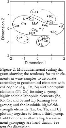
DATA
9 Trace-element behavior in the wine dataset is not random. First, the highfield strength lithophile elements, U, Th, La and Ce plot close together on the MDS diagram (Fig. 2) indicating similar behavior. "Similar behavior" means that the concentrations of these trace elements are positively correlated in the wines and an X-Y plot (not shown) of the concentrations of any two elements, in all wines, would yield a straight line with a high correlation coefficient. Thus, when one of these high-field strength lithophile elements is present in large amounts (or small amounts) in a wine, all such elements tend to be present in large (or small) amounts. Second, the large ion lithophile elements form two groups on opposite sides of Figure 2, also suggesting coupled behavior: When Sr and Li are present in large amounts; Cs, Rb and Ba tend to be present in small amounts, and vice versa. Third, the chalcophile (Cu, Pb, Zn, Cd, Mo, As,Ag, Bi) and siderophile elements (Ni, Co) form a large group occupying the middle of the diagram.
Table 1: Information on climate, soil and bedrock contributing to the terroir of Canadian viticultural regions.
Display large image of Table 1
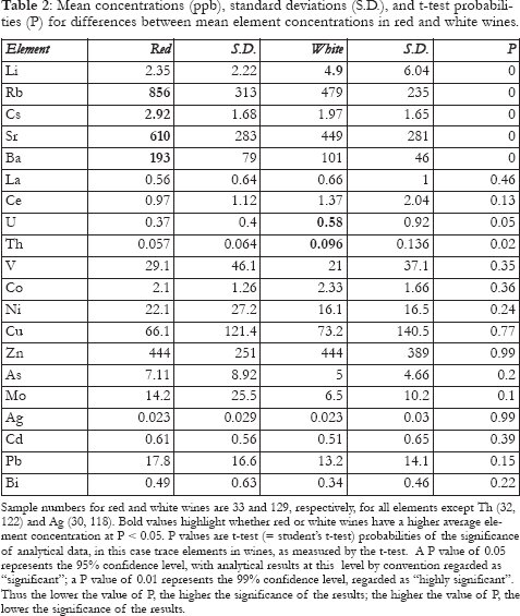
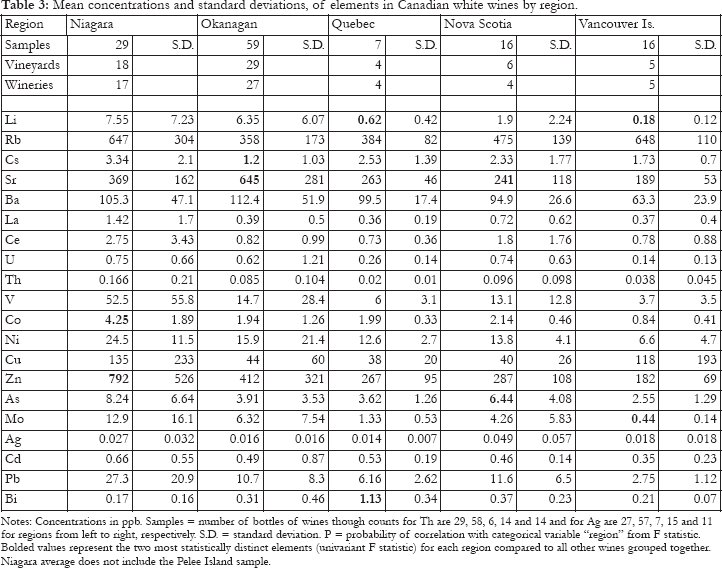
10 On average, the red wines have significantly higher concentrations of Rb, Cs, Sr and Ba, than the white wines (P < 0.05, where P = t-test probability; see Table 2 for values and brief explanation of probability factor, P); whereas the white wines have higher Li, U and Th (bolded values, Table 2). Because wine colour and composition are related, Table 3 compares the regional average compositions of only the white wines, the largest dataset. P values (right column) indicate that the average concentration of nearly all trace elements is strongly correlated with region (P <0.05). Niagara region white wines have the highest average concentrations for most trace elements. Exceptions are the high Sr and Ba concentrations in Okanagan wines. Okanagan wines also have the smallest amounts of Cs. In contrast with Niagara, Vancouver Island wines have either the lowest or second lowest average concentrations of nearly all trace elements. Bolded values in Table 3 point out the two elements from each region with mean concentrations that are statistically distinct.
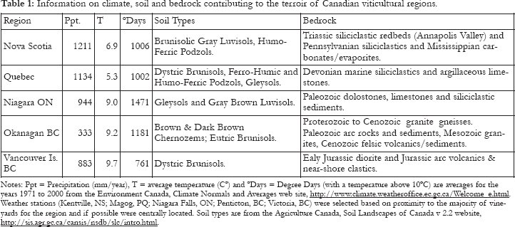
11 Figures 3a and 3b provide 3-D, MDS "maps" of white and red wine trace-element sample relationships. Samples plotting close together are very similar in trace-element compositions. To understand how "similarity" is determined for wines, imagine a graph (not shown) with all trace-element concentrations in one wine plotted against all concentrations in a similar wine (i.e., two wines close together in Fig. 3). The two wines would produce a straight line graph with a high correlation coefficient. MDS arranges samples using a set (matrix) of correlation coefficients that measure (estimate) the distances between all possible pairs of wines. Stated another way, the MDS coordinates for a single wine (Fig. 3) are determined from the estimated distances to all other wines, a procedure something like locating the epicentre of an earthquake by using three or more seismic stations. Finally, instead of determining "distances" between samples in two dimensions, as done for elements in Figure 2, coordinates were determined in three dimensions, analogous to longitude, latitude and depth in the Earth. Because three-dimensional relationships are difficult to portray in two-dimensional diagrams on paper, sample coordinates are projected onto the Dimension 1 versus Dimension 2 plane (Fig. 3a), and Dimension 1 versus Dimension 3 plane (Fig. 3b).
Figure 3. Multidimensional scaling diagrams showing relationships between wine samples in three dimensions. Symbols O = Okanagan, V = Vancouver Island, S = Nova Scotia, N = Niagara including two Pelee Island samples, Q = Quebec. The hand-drawn field in Figure 3a encompasses 90% of the red wine samples of this study. Dimension 2 predominantly reflects the impact of wine colour on composition. Hand-drawn fields in Figure 3b show that wine trace-element compositions reflect region of origin. Okanagan wines plot apart from most other wines along Dimension 1, and apparently represent the predominant source of chemical variation in the data set. Chemical differences between Niagara, Vancouver Island and Quebec samples are summarized along Dimension 3, but Nova Scotia samples appear to have less-distinct compositions.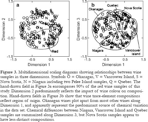
Display large image of Figure 3
Display large image of Figure 4
12 The hand-drawn field in Figure 3a encompasses 90% of the trace-element compositional variability of all red wines of this study, but only 17% of the trace-element compositional variability of the white wines, indicating that Dimension 2 reflects the impact of wine colour on trace-element composition. The labeled fields in Figure 3b encompass ~ 90% of the trace-element compositional variability of wine samples from the Okanagan Valley, Quebec, Niagara and Vancouver Island with little overlap. Nova Scotia wines show more overlap with other regions, but most samples fall close to the Vancouver Island field. It is apparent that Dimensions 1 and 3 express differences in wine trace-element composition controlled by region-of-origin. In summary, Figure 3 diagrams indicate that wine colour and region-of-origin represent the two predominant factors controlling wine composition.
DISCUSSION
Trace Element Compositions of Red and White Wines
13 Our results confirm that red and white wines have distinct trace-element compositions (Greenough et al., 1997; Baxter et al., 1997). Elements that have significantly different (P < 0.05) average concentrations include Rb, Cs, Sr and Ba, which are higher in red wines; and Li, U and Th which are higher in white wines (Table 2). Greenough et al. (1997) reported similar results: Ba, Mo, Ca, P and Mg were significantly higher in red wines (P < 0.05) with Li higher in white wines. Average Rb, Cs and Sr concentrations were also reported higher in reds, and U lower, but the differences were not as large (significant) as for Ba, etc. Combining study results, red wines have higher Rb, Cs, Sr, Ba and Mo, and white wines higher Li, U and Th concentrations.
14 The differences among wine types (varietal or hybrid) could reflect trace-element concentrations in grapes. However, there are no other known relationships between grape variety and trace-element concentrations, and the trace-element differences between red and white wines apply to Vitis vinifera and non-Vitis vinifera (e.g., hybrid) varieties alike. That is, they apply to grapes with genetic differences arguably more fundamental than those relating to colour. One wine, a blush wine made from red wine grapes (Pinot Noir) and processed in a white wine style, plotted with white wines on the MDS diagram (Fig. 3). Thus trace-element differences between red and white wines do not appear to be related to grape variety.
Effects of Processing
15 The inorganic composition of wine undoubtedly is affected by how wines are produced. Bentonite, a fining (clarifying) agent, can increase rare-earth-element concentrations (Jakubowski et al., 1999), and storage of wine in stainless steel vats may raise Ni and Fe content in such wines (Eschnauer, 1982; Murányi and Papp, 1997). The addition of K or Na metabisulfite to wines to control oxidation and microbial activity (Cox, 1985), the natural precipitation of K bitartrate (wine diamonds), storage in oak casks (that add organic compounds; Eggers et al. in press ), or contact with the bottle's cork may also affect trace-element concentrations (Taylor et al., 2002). Whether some of these factors can account for differences between red and white wine trace-element compositions is explored below.
Table 2 : Mean concentrations (ppb), standard deviations (S.D.), and t-test probabilities (P) for differences between mean element concentrations in red and white wines.
Display large image of Table 2
16 Differences in alkalis (Na, K) might be caused by the precipitation of K bitartrate but this occurs in both red and white wines, and does not explain differences in high-field-strength elements such as U, Th, La, and Ce. Higher alkali and alkaline-earth-element concentrations in red wines could reflect the addition of Na or K metabisulfite. However, metabisulfite use is not ubiquitous; yet, as pointed out above, the same trace-element compositional differences between red and white wines turn up from one study to another. Also, metabisulfite addition cannot explain lower Li and high-field-strength elements in red wines. The Sr isotopic composition of wines closely reflects soil composition (Barbaste et al., 2002) indicating that little Sr is added to wine during processing. This argues against metabisulfite as a source for Sr. Finally, metabisulfite is used more extensively with white wines. Thus, higher alkali and alkaline earth-element concentrations in red wines appear to be unrelated to matabisulfite addition.
17 Bentonite is apparently more commonly used as a fining agent in white wines than in red wines. Its use raises rare-earth-element concentrations (Jakubowski et al., 1999) and might similarly affect other high-field-strength elements. If so, bentonite would also have to adsorb Rb, Cs, Sr, Ba and Mo, and release Li, to explain the other differences between red and white wines. However, this explanation has problems. Average Niagara and Vancouver Island red and white wines show the same relative pattern of Rb, Cs, Sr, Ba, Mo, Li, U and Th enrichment/depletion as is seen in the dataset (Table 2). Both red and white Niagara wines have higher concentrations of all trace elements than Vancouver Island wines. These regional differences in composition would be difficult if not impossible to preserve if bentonite addition has had a major impact on wine chemistry. Similar arguments can be made that less-common or non-ubiquitous addition of fining agents such as egg albumin, isinglass (= gelatin; more commonly used with red wines) and casein (= milk protein; more commonly used with white wines), have minimal impact on wine trace-element chemistry. The same can be said for oaking and cork effects.
Table 3: Mean concentrations and standard deviations, of elements in Canadian white wines by region.
Display large image of Table 3
18 The simplest explanation for trace-element concentration differences between red and white wines is that contact between grape skins, seeds and must (juice) during red wine fermentation affects the extraction of highly soluble elements (e.g., Rb, Cs) that are metabolically concentrated in skins or seeds during growth. Under this hypothesis, Li and highly insoluble elements including U, Th, La and Ce are absorbed by the damaged skins. The end result is differences in element concentrations between red wines and white wines that also preserve or reflect regional compositional differences.
Regional Differences in White Wine Trace-Element Composition
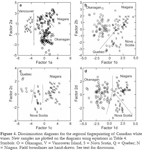
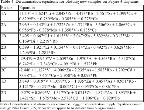
19 As noted previously, only white wine trace-element concentrations are used here to discuss regional differences in composition. P values given in Table 3 show that nearly all trace elements in the white wines are highly correlated with "region of origin". Bolded values highlight two of the more distinct elements for each region, but regions should be more accurately distinguished using combinations of elements. Figure 4 shows how Canadian white wines could be regionally "fingerprinted". These discriminant analysis diagrams use multiple elements from the dataset to visually separate samples by region. The statistical output includes equations (Table 4) that allow new samples, of unknown origin, to be classified. All equations in Table 4 use ≤ 10 elements.
20 Trace-element concentrations for a new wine are converted to a Log10 format and inserted into Table 4 equations. The calculated Factor values (Table 4) are plotted on the diagrams of Figure 4a to d.
21 The hand-drawn vertical line in Figure 4a separates Vancouver Island white wines with 100% accuracy. Non-Vancouver Island white wines are plotted on Figure 4b, which divides samples into two groups for plotting on Figures 4c and 4d. The hand-drawn field lines in Figure 4c separate Quebec, Nova Scotia and Niagara wines in our dataset with 100% accuracy. The hand-drawn field lines shown in Figure 4d leave only 4 of 104 samples from the Okanagan, Niagara and Nova Scotia incorrectly classified.
22 The efficiency of separation shown in Figure 4 may be optimistic, however, owing to limited numbers of white wine/trace-element samples from some of the regions of this study. Niagara and Okanagan separations appear rigorous because they are based on many white wines from numerous vineyards. Quebec, in contrast, is represented by only seven samples from four vineyards (Table 3). Nevertheless, numerous possible diagrams and combinations of elements (not shown) yield similarly accurate classifications. Separations tend to be more effective -fewer samples are incorrectly classified – when larger numbers of trace elements are used. From a geological and analytical perspective this is reasonable, because more elements filter out variation of unknown origin (randomness) and ameliorate analytical error. However, with small numbers of samples (e.g., Quebec), large numbers of elements increase the likelihood that the classification procedure will only work with the original samples. New samples may be incorrectly classified.
23 Many studies suggest that wines can be fingerprinted with trace-element data at the vineyard level through to regional level (Latorre et al., 1994; Stroh et al., 1994; Day et al., 1995; Greenough et al., 1996; 1997; Baxter et al., 1997; Danzer et al., 1999; Taylor et al., 2002; 2003; Diaz et al., 2003). Although wine isotopic ratios reflect soil ratios (Barbaste et al., 2002), absolute element concentrations are difficult to relate to soil or bedrock compositions (Greenough et al., 1996; Taylor et al., 2002). As with plants, however (Brooks, 1972, p. 96-99), absolute concentrations of individual elements in wines correlate with solubility in water (predicted from ionic potential, = charge/radius ratios). Elements such as La and Ce show low concentrations in wines compared to soils and rocks because these elements are insoluble, whereas elements such as Rb and Sr are present in higher concentrations owing to higher solubility in water (Greenough et al., 1996). Also, studies of Okanagan wines have shown that trace-element concentrations correlate qualitatively with a climate gradient between the south (hot and dry) and north (more-temperate and wetter) ends of the valley (Greenough et al., 1997; Taylor et al., 2002).
24 Figure 2 provides clues to the causes of regional differences in the composition of Canadian wines. When data from several unrelated chemical systems (e.g., random analyses of unrelated rocks) are examined with multidimensional scaling, trace elements tend to plot randomly (e.g., Mallory-Greenough et al., 1998). Non-random behaviour (e.g., Fig. 2) implies that similar geochemical processes are controlling trace-element behaviour in the wines. Because many different rocks underlie vineyards, if bedrock had a predominant influence on wine chemistry, trace-element behaviour in Figure 2 should be more random. Further, the separation of soluble from insoluble lithophile elements in the dataset suggests that climate-related weathering and element solubility are important factors in determining trace-element concentrations in wines (Greenough et al., 1996). Bedrock composition may help to distinguish wines at the vineyard level, but for regional discrimination of wines it is likely of secondary importance. Note, however, that this conclusion does not apply to isotopic ratios.
Table 4: Discrimination equations for plotting new samples on Figure 4 diagrams.
Display large image of Table 4
25 Tables 1 and 3 and Figure 5 suggest further links between climate and wine composition. Vancouver Island wines show low average concentrations of most trace elements whereas the highest concentrations occur in Niagara wines. Except for Bi, all averaged element data (Table 3) have a positive correlation with climate-related Degree Days (Table 1). In fact, 14 of 20 trace elements show a correlation coefficient (r) with Degree Days of > 0.74 (P <0.15) and eight (Li, V, Co, Ni, Zn, Mo, Cd, Pb) have r > 0.91 (P < 0.03; and e.g., Fig. 5)! One explanation for this feature may be that higher temperatures lead to higher solubility of elements in soils. An alternative explanation may be that areas with higher Degree Day values - warmer temperatures - yield greater evaporative losses leading to more water uptake by grapes, thus increasing trace-element concentrations in grapes. This second hypothesis is supported by the linear, arithmetic relationships between trace-element concentrations and Degree Days, and by somewhat similar concentration factors [geometric mean and standard deviation = 8.5 + 2.9 times; range = 41 (Li) to 1.9 (Cd) times] for these elements between Vancouver Island and Niagara (Table 3). Rb, Cs and Sr correlate poorly with Degree Days (r < 0.55; P < 0.35), and Okanagan wines have high Sr concentrations (Taylor et al., 2002). This may reflect the concentration of alkaline earth metals (Ca, Sr) in soil and groundwater as is typical in dry climates.
26 Regardless of the underlying causes, there are strong regional variations in the trace-element composition of Canadian wines. Our dataset includes 20 trace elements, but the ICP-MS is capable of routinely determining more than 40 elements. Considering that nearly all 20 trace elements reported here are highly correlated with "region", other trace elements should be similarly useful. With a larger sample base, assembled over several years, more trace elements could be "safely" used in discrimination. In addition, ICP-MS isotopic data promise to become routinely available, providing more discriminating power as indicated by experiments fingerprinting Italian and French wines (Day et al., 1995; Barbaste et al., 2002; Larcher et al., 2003). Still, there are unresolved issues. For example, ice wines and late harvest wines appear to have anomalous compositions compared to "normal" wines from the same vineyard.
27 Will trace-element fingerprinting become part of the Vintners Quality Alliance (VQA) certification procedure for wines? Undoubtedly ICP-MS analysis of trace elements can provide routine, accurate and inexpensive data and, as shown here, such analyses are capable of separating wines by region with a high degree of accuracy. There are, however, potential legal ramifications to incorrectly classifying a wine. Whether analytical and statistical methods can be refined, or regulations written with limitations in mind, remains to be seen. For now it is clear that there are academic and potential private uses for wine fingerprinting.
Figure 5. Plot of Degree Days versus the average concentrations of selected elements in wines from each of the Canadian wine producing areas. Concentrations are highly correlated with Degree Days. See text for discussion. Symbols as in Figure 4.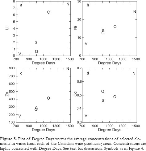
ACKNOWLEDGEMENTS
We acknowledge the many viticulturalists and wine makers across Canada who helped with sample selection. H. Soon (Sandhill), G. Stanley (Quails Gate), and D. Barnett (Lailey) advised on wine-making practices. H. Muggeridge and R. Corney prepared the diagrams. We are grateful for critical reading by Georgia Pe-Piper and Roger Macqueen; their comments improved presentation of the paper. This research was in part supported by NSERC research grants to JDG and BJF.REFERENCES
Barbaste, M., Robinson, K., Guilfoyle, S., Medina, B., and Lobinski, R., 2002, Precise determination of the strontium isotope ratios in wine by inductively coupled plasma sector field multicollector mass spectrometry (ICP-SF-MC-MS): Journal of Analytical Atomic Spectrometry, v. 17, p. 135-137.
Baxter, M.J., Crews, H.M., Dennis, J.M., Goodall, I. and Anderson, D., 1997, The determination of the authenticity of wine from its trace element composition: Food Chemistry, v. 60, p. 443-450.
Borg, I. and Groenen, P., 1997, Modern Multidimensional Scaling, Theory and Applications: Springer-Verlag, New York, 471 p.
Bowen, P.A., Bogdanoff, C.P., Estergaard, B.F., Marsh, S.G., Usher, K.B., Smith, C.A.S., and Frank, G., 2005, Use of Geographical Information System technology to assess viticultural performance, Okanagan and Similkameen valleys, British Columbia: Geoscience Canada, v. 32, no.4, In press.
Brooks, R.R., 1972, Geobotany and Biogeochemistry in Mineral Exploration: Harper and Row, New York, 290 p.
Cox, J., 1985, From Vines to Wines: Harper and Row, New York, 253 p.
Danzer, K., De La Calle Garcia, D., Thiel, G. and Reichenbacher, M., 1999, Classification of wine samples according to origin and grape varieties on the basis of inorganic and organic trace analyses: American Laboratory, v. 31, p. 26-33.
Day, M.P., Zhang, B. and Martin, G.J., 1995, Determinatoin of the geographical origin of wine using joint analysis of elemental and isotopic composition. II Differentiation of the principle production zones in France for the 1990 vintage: Journal of the Science of Food and Agriculture, v. 67, p. 113-123.
Davis, R., Chilton, R., Ottenbreit, L., Scheeler, M., Vielvoye, J., Williams, R. and Wittneben, U., 1984, Atlas of Suitable Grape Growing Locations in the Okanagan and Similkameen Valleys of British Columbia: Agriculture Canada, Summerland, British Columbia, 141 p.
Diaz, C., Conde, J.E. and Estevez, D., 2003, Application of multivariate analysis and artificial neural networks for the differentiation of red wines from the Canary Islands according to the island of origin: Journal of Agricultural and Food Chemistry, v. 51, p. 4303-4307.
Eggers, N., Greenough, J.D. and Cernak, T., in press, Identifying the Terroir of Okanagan Valley, British Columbia, Chardonnay Wines Using Volatile Components: Geoscience Canada reprint volume, Geology and Wine.
Eschnauer, H., 1982, Trace elements in must and wine: primary and secondary contents: American Journal of Enology and Viticulture, v. 33, p. 226-230.
Fulton, R.J., 2003, Geology of Okanagan Valley wine region of British Columbia. [Abstract]: 2003 Seattle Annual Meeting of the Geological Society of America, Paper 74-2.
Grant, E.B., Ker, K. and Haynes, S., 2004, Niagara Geology and Wine: Fieldtrip Guidebook, Geological Association of Canada - Mineralogical Association of Canada, Joint Annual Meeting 2004, Brock Univ., St. Catharines, ON, 17 p.
Greenough, J.D., Longerich, H.P. and Jackson, S.E., 1997, Element fingerprinting of Okanagan Valley wines using ICPMS: Relationships between wine composition, vineyard and wine colour: Australian Journal of Grape and Wine Research, v. 3, p. 75-83.
Greenough, J.D., Longerich, H.P. and Jackson, S.E., 1996, Trace element concentrations in wines by ICP-MS: Evidence for the role of solubility in determining uptake by plants: Canadian Journal of Applied Spectroscopy, v. 41,p. 76-80.
Greenough, J.D., Lutmerding, H., and Mallory-Greenough, L., 2004, Chapter 7, Geology and terroir of Okanagan Valley wine: in Roed, M. and Greenough, J.D., eds., Okanagan Geology, Kelowna Geology Committee, Kelowna, BC, p. 67-70.
Haynes, S.J., 1999, Geology and Wine 1. Concept of Terroir and the Role of Geology: Geoscience Canada, v. 26, p. 190-194.
Haynes, S.J., 2000, Geology and Wine 2, A geological foundation for terroirs and potential for sub-appellations of Niagara Peninsula wines, Ontario, Canada: Geoscience Canada, v. 27, p. 67-87.
Jakubowski, N., Brandt, R., Stuewer, D., Eschnauer, H.R. and Gortges, S., 1999, Analysis of wines by ICP-MS: Is the pattern of the rare earth elements a reliable fingerprint of provenance?: Fresenius Journal of Analytical Chemistry, v. 364,p. 424-428.
Johnson, H., 1991, Hugh Johnson's Modern Encyclopedia of Wine: Simon and Schuster, New York, 576 p.
Larcher, R., Nicolini, G. and Pangrazzi, P., 2003, Isotope ratios of lead in Italian wines by inductively coupled plasma mass spectrometry: Journal of Agricultural and Food Chemistry, v. 51,p. 5956-5961.
Latorre, M.J., Garcia-Jares, C., Medina, B. and Herrero, C., 1994, Pattern recognition analysis applied to classification of wines from Galicia (northwest Spain) with certified brand of origin: Journal of Agriculture and Food Chemistry, v. 42, p. 1451-1455.
Mallory-Greenough, L.M., Greenough, J.D. and Owen, J.V., 1998, New data for old pots: Trace element characterization of ancient Egyptian pottery using ICP-MS: Journal of Archaeological Science, v. 25,p. 85-97.
Murányi Z. and Papp L., 1997, ICP-AES metal content analysis of wines made with different technologies: ACH-models in Chemistry, v. 134 p. 529– 537.
Rollinson, H., 1993, Using Geochemica Data: Evaluation, Presentation, Interpretation: Longman, Essex, England, 352 p.
Stroh, A., Brückner, P. and Völlkopf, U., 1994, Multielement analysis of wine samples using ICP-MS: Atomic Spectroscopy, v. 15, p. 100-106.
Tabachnick, B.G. and Fidell, L.S., 2001, Using Multivariate Statistics, 4th edition: Allyn and Bacon, Toronto, 966 p.
Taylor, V.F., Longerich, H.P. and Greenough, J.D., 2002, Geology and Wine 5. Provenance of Okanagan Valley wines, British Columbia, using trace elements: promise and limitations: Geoscience Canada, v. 29, p. 110-120.
Taylor, V.F., Longerich, H.P. and Greenough, J.D., 2003, Multielement analysis of Canadian wines by inductively coupled plasma mass spectrometry (ICP-MS) and multivariate statistics: Journal of Agricultural and Food Chemistry, v. 51,p. 856-860.
Wilkinson, L., Hill, M., Welna, J.P. and Birkenbeuel, G.K., 1992, SYSTAT for Windows: Statistics, Version 5 Edition: SYSTAT Inc., Evanston, IL, 750 p.