Series
Google Earth® Models with COLLADA and WxAzygy® Transparent Interface:
An example from Grotto Creek, Front Ranges, Canadian Cordillera
Co-author Scott Shipley has posted supplemental files to YouTube, collectively at: http://www.youtube.com/user/WxAzygy?ob=0&feature=results_main
Specific files of note for this article are located on the GAC open access site: Canada GEESE Series: http://www.gac.ca/wp/?page_id=6991
SUMMARY
Virtual globes represent a paradigm shift for geoscience education. It is now possible to explore real world experiences across the entire Earth, the Moon, and Mars, and also to combine multiple 2-D images into one 3-D image with topography. Models viewed in Google Earth® are more intuitive for visualizing 3-D geological structures than traditional paper maps and cross-sections. Here a student-constructed geological map and cross-sections from an introductory field school are used to illustrate the creation of a draped geological map over topography. A custom vertical slider elevates the cross-sections above topography and a horizontal slider restores thrust faulting. Models located in situ in topography are made queryable via a ‘cut-away’ using the WxAzygy® transparent interface.
SOMMAIRE
La notion de « globes virtuels » constitue un changement de paradigme dans le domaine de l’éducation en géo-science. Il est maintenant possible de traiter de la réalité de tous les recoins de la Terre, de la lune et de Mars, et aussi de combiner de multiples images 2-D en une image 3-D affichant la topographie. Les modèles de Google Earth® permettent une visualisation 3-D plus intuitive des structures géologiques que ne le permettent les cartes papiers usuelles et les coupes. Dans la présente, une carte géologique et une coupe réalisées par un étudiant d’un cours d’introduction au travail de terrain sont utilisées pour illustrer la confection d’une carte géologique appliquée sur la topographie correspondante. Un curseur vertical personnalisé dessine les coupes au-dessus de la topographie, et un curseur horizontal permet de restaurer les failles de chevauchement. Ces modèles ancrés au droit de la topographie peuvent être exploiter au moyen d’un écorché produit par l’interface transparent WxAzygy®.
INTRODUCTION TO Google Earth® MODELS AND VIRTUAL FIELD TRIPS
1 Google Earth® and other virtual globes have only been available for a decade, yet they represent a significant paradigm shift for geoscience education. Now it is possible for students (agile and disabled) to explore the entire Earth, Moon, and Mars. In Google Earth®, these students can also be exposed to real-world type experiences, rather than a typical ‘canned laboratory’ exercise. Here a Google Earth® model is presented that provides some interactive components critical for creating excellent virtual field trips (VFTs, Hurst 1997; Woerner 1999; Tuthill and Klemm 2002; Arrowsmith et al. 2005).
2 As outlined by Mogk (2011), the novice geology student is impacted by multiple factors such as distraction by irrelevant features (Goodwin 1994; Reynolds et al 2006), spatial and scale relations (Wilson 2001, 2002; Montelo et al 2004), internal versus external views (Bryant et al. 1992), and the affective domain (values, motivations, emotions, attitudes, etc; Krathwohl et al 1973) all of which cause the first field experience to be overwhelming. A VFT is best employed as a supplemental introduction to real field experiences (Bellan and Scheurman 2001; Tuthill and Klemm 2002; Arrowsmith et al. 2005; Smedley and Higgins 2005) and could potentially lessen the overwhelming nature of first field experiences.
3 Virtual globes emerged at the close of the last millennium (Bailey 2000). Gore (1998) strongly endorsed this technology and predicted that virtual globes would revolutionize spatial visualization and data analysis for geo-science research and education. Earth-browser was the first working digital globe application to appear in 1998, followed by other ‘first generation’ virtual globes until 2004. Development of the XML-based markup language ‘Keyhole Markup Language’ (KML) by Keyhole Corporation in the early 2000s made virtual globes easily extensible. Google Earth® was released in 2005 as the newly named KML-based geobrowser (after Google Inc. purchased Keyhole Inc.). Google ensured the success of Google Earth® by releasing control of KML to the Open Geospatial Consortium in 2008, thereby establishing KML as the standard for interactive digital globes. KML is now the scripting language for all major virtual globes such as ESRI’s Arc Explorer, Bing Maps 3-D (formerly MSN Virtual Earth), Google Earth®, and NASA’s World Wind (Wilson et al. 2007, 2008; Wernecke 2009; Whitmeyer et al. 2010; De Paor et al. 2010; De Paor and Whitmeyer 2011).
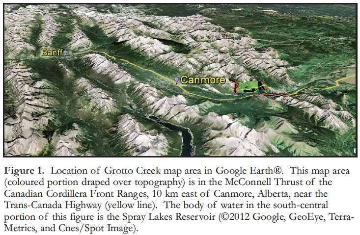
4 Google Earth® capabilities were greatly expanded with the adoption of COLLADA (COLLAborative Design Activity) for 3-D content modelling in 2006 (with version 4), and Animation in 2007 (with version 5). COLLADA was originally developed by Sony Entertainment Corporation for exchange of 3-D graphics content (Arnaud and Barnes 2006). It is now an open standard maintained by Khronos Group (Khronos Group 2012). Google developed SketchUp (which it recently sold to Trimble Navigation Inc.) as a user-friendly application for creation of 3-D content, such as buildings. SketchUp version 8 was used in this paper to create emergent COLLADA models of subsurface structures and to animate COLLADA models with the Google Earth® Application Program Interface (API) and JavaScript (De Paor and Whitmeyer 2011). Emergent and animated COLLADA models are presented here using the Grotto Creek mapping project from an introductory field school taught at Mount Royal University, Calgary, Alberta, Canada (Fig. 1).
 Display large image of Figure 1
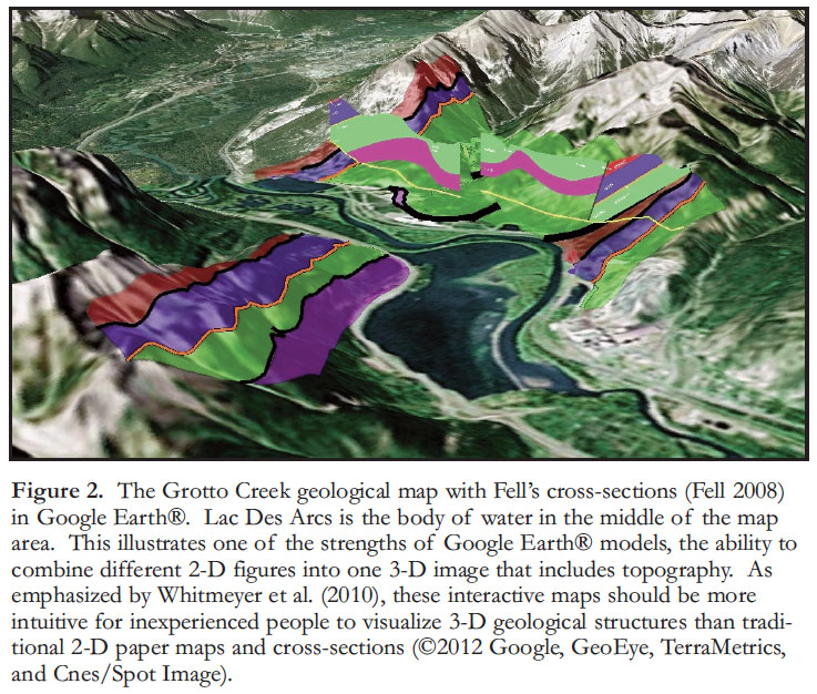
5 The Grotto Creek exercise (Fig. 2) was initially created for education, to guide novice geology students while developing the necessary spatial cognitive abilities during their voyage toward becoming professional geologists. Novice students and non-professionals typically experience difficulties when attempting to visualize 3-D geological structures with paper geologic maps and cross-sections (Piburn et al. 2002; Kastens and Ishikawa 2006). As emphasized by Whitmeyer et al. (2010), interactive geological maps in Google Earth® communicate 3-D geological data more intuitively than the traditional format of separate paper maps and cross-sections. Draping geological maps over topography combined with creating emergent cross-sections permits students to remove much of the cognitive barrier involved in trying to piece together 2-D paper maps and paper cross-sections.
 Display large image of Figure 2
6 Using the method of Dordevic (in press), multiple slider controls can be created for the Google Earth® API that are controlled using JavaScript code. Here a vertical slider was used to create emergent cross-sections, while a horizontal slider recreates the formation of the faults and folds observed in the field area. In a further innovation, WxAnalyst’s WxAzygy® Transparent Interface (Shipley et al. 2009, 2010) was used to create a queryable ‘cut-away’ cross-section into the topography. The main purpose of this paper is to highlight the practical and accessible nature of Google Earth® when combined with SketchUp, COLLADA, and WxAzygy®, and the ability to create engaging 3-D interactive models from geological maps and cross-sections constructed by students or professionals.
THE GROTTO CREEK MAPPING PROJECT
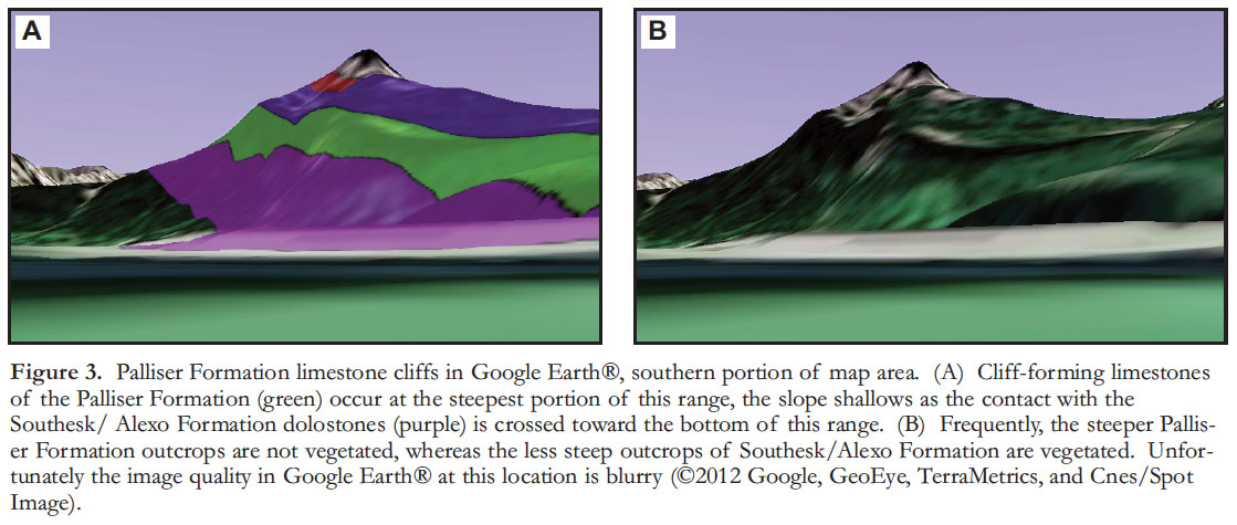
7 The Grotto Creek map area is located in the McConnell Thrust Sheet in the Front Ranges of the Canadian Cordillera, near the Trans-Canada Highway between Calgary and Banff, Alberta (Fig. 1). Devonian–Mississippian carbonate–clastic strata were deposited on the western margin of ancestral North America and then repeated by folding and faulting along the Lac des Arcs Thrust Fault. The >440 m thick Devonian to Carboniferous stratigraphic sequence in the Grotto Creek map area progresses from the shelf margin wedge systems that onlapped bathymetric highs in Alberta during a sea-level rise (Southesk/Alexo and Palliser formations, Fig. 3A, B), to the transgressive systems tract of the Exshaw Formation (Caplan and Bustin 1996, 1998). This was accompanied by eutrophication of surface waters and reduced carbonate accumulation rates with the destruction of the carbonate platform due to changes in the paleoceangraphic circulation marked by the black organic-rich shales of the lower member of the Exshaw Formation. The bioturbated shelf siltstones and cross-stratified nearshore marine sandstones of the upper member of the Exshaw Formation record an abrupt relative sea-level fall (Caplan and Bustin 1996, 1998) that continued through to the development of a second carbonate platform represented by the Banff and Livingstone formations.
 Display large image of Figure 3
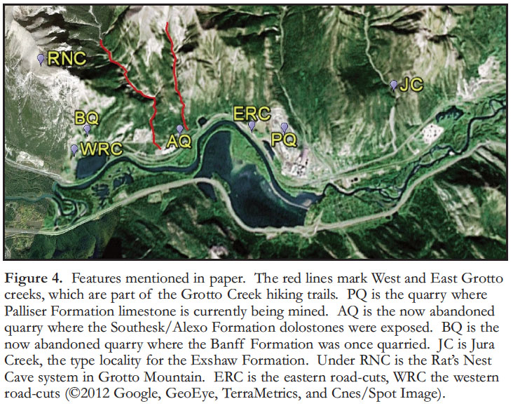
8 This mapping project was chosen because the five mapped formations are important to the local petroleum industry in the Western Canadian Sedimentary Basin. For example, the Exshaw Formation (Allan and Creaney 1991; Barson et al. 2000; Manzano-Kareah et al. 2004 and multiple references therein) is an important source rock for many petroleum reservoirs in Western Canada. The clean and pure limestone of the Palliser Formation is quarried in the map area for cement. Karst topography within the Livingstone Formation formed the Rat’s Nest Cave system (Yonge 2001) in Grotto Mountain. The cliff-forming limestone of the Palliser and Livingstone formations form the spectacular landscapes that draw millions of tourists to our geological backyard. Access into this area is excellent with road-cuts along Highway 1A and popular hiking trails up the two Grotto creeks. West Grotto Creek follows one of the syncline hinge lines, while East Grotto Creek cuts up the trace of a small thrust fault.
9 Jonathan Fell (Fell 2008) constructed the geological map and the two shorter cross-sections used here (Fig. 2), during his introductory field school at Mount Royal University (Calgary, Alberta). As per many Canadian B. Sc. geology major programs, the introductory field school is taught for two weeks during the end of summer before the second year geology courses. The Grotto Creek field area represents the final four-day mapping project of the field school.
10 Four days were spent mapping the toe of Grotto Mountain, west and east Grotto creeks and the road-cuts along Highway 1A in the western portion of the field area (see Fig. 4 for geographic features mentioned throughout this paper). Two stops were made at outcrops along the southern side of the Trans-Canada Highway to include those on the map and to examine the structural features of the mapping area from a distance. A stratigraphic column was measured along Highway 1A road-cuts in the eastern portion of the map area earlier in the field school. Two days were spent in Jura Creek (2.7 km northwest of the mapping area) mapping the top and bottom contacts of the Palliser and Exshaw formations. Jura Creek is the type locality for the Exshaw Formation (MacQueen and Sandberg 1970; Barson et al. 2000) which is recessive and eroded away within the Grotto Creek area. To complete the map and to practice structural contouring, the contacts were structurally contoured north and south of the out-crops.
11 Due to time constraints, the region between the East Grotto Creek thrust fault and the Lac des Arcs thrust fault was not visited (Fig. 4). To complete the geological map, the students were asked to extrapolate the geology from the final mapping project area (western portion) to the eastern road-cuts. So, while this geological map does include the anticline–syncline pair (West Grotto Creek) and the small thrust fault (East Grotto Creek) added by Simony (in Spratt et al. 1995) to the McMechan (1995) and Price (1970) geological maps for this region, the portion between the two thrust faults does not correspond to the work of Price (1970), McMechan (1995) and Simony (in Spratt et al. 1995) because the students were not aware of this work. These differences are not the focus of this paper, rather we aim to highlight how student mapping can be enhanced and presented in an engaging 3-D interactive setting using Google Earth®, COLLADA and WxAzygy®.
 Display large image of Figure 4
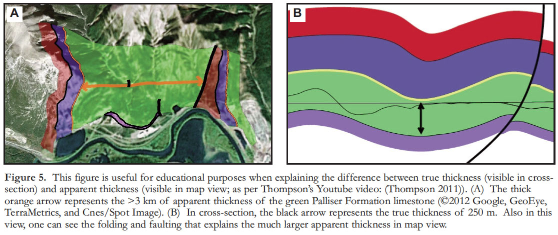
12 Robyn Thompson (Instructional assistant at Mount Royal University), digitized Fell’s map and cross-sections (Fell 2008), and used these to create an emergent model and terrain overlay using SketchUp and KML code. Thompson used an early version of the Grotto Creek model to create a Youtube video (Thompson 2011) illustrating the difference between the >3 km apparent map thickness of the green Palliser Formation limestone and the ~250 m true thickness observed in the cross-sections (Fig. 5A, B). This illustrates one powerful capacity for these Google Earth® models for education purposes.
 Display large image of Figure 5
13 This Grotto Creek Google Earth® model will be used in introductory geology courses to illustrate the ‘rule of Vs’ and why inclined contacts are not always straight lines. The terrain overlay combined with the topography in Google Earth® greatly enhances what may be difficult for some students to visualize with only the topographic contours on topo-graphic maps. Thompson’s Youtube video (Thompson 2011) will be used in the introductory field school, and structural geology courses to graphically illustrate the difference between true and apparent thickness. The vertical and horizontal sliders will be used in these courses to illustrate how folds and faults can develop and how to construct proper cross-sections. Both concepts can be troublesome for novice students.
14 Perhaps the most powerful application of Google Earth® models for the geosciences is in the creation of interactive components to create effective virtual field trips (VFTs; Hurst 1997; Woerner 1999; Tuthill and Klemm 2002; Arrowsmith et al. 2005). Most geology students are completely overwhelmed during the first day of introductory field schools due to factors listed above – distraction by irrelevant features, spatial and scale relations, internal versus external views, and the affective domain. Student responses in Arrowsmith et al. (2005) support the conclusion that VFTs assist students in preparing for fieldwork and that most students felt more comfortable during the real field experience after being exposed to a VFT. These same students also mentioned that VFTs should not replace real field experiences. The Grotto Creek Google Earth® model presented here represents the first stage of creating a much larger VFT through the Canadian Cordillera.
EMERGENT COLLADA MODELS AND STRUCTURAL RECONSTRUCTIONS
Stage Design for the Grotto Creek Model
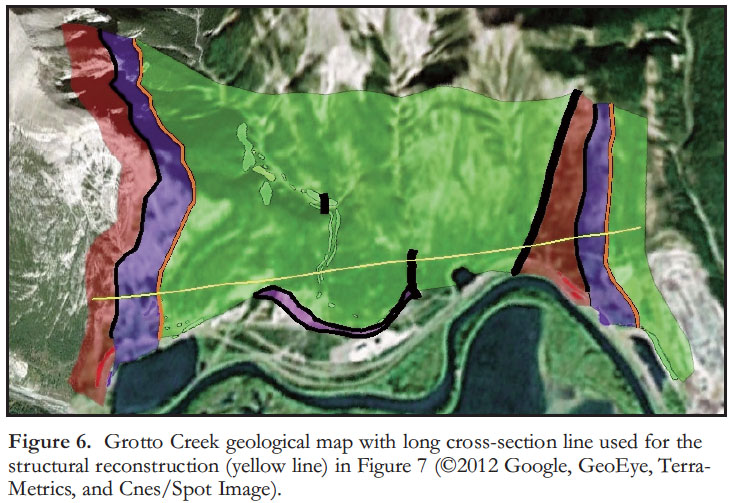
15 The senior author created the longer cross-section (Fig. 6) and stages for the structural emergent model (Fig. 7) from Fell’s field school geological map (Fell 2008). As emphasized by Enkin et al. (1997, 2000), extensive mapping and structural analysis has outlined the architecture of the Front Ranges (Clark 1949; Bally et al. 1966; Dahlstrom 1970; Price 1970; Price and Mountjoy 1970; Monger and Price 1979; Price 1994; McMechan 1995; Simony in Spratt et al. 1995), however the timing, mechanism and environment of Cordilleran deformation remain incompletely understood. Wheeler et al. (1974) proposed that approximately 140 km of shortening in the Front Ranges occurred at a rate of ~2 mm/yr between Early Cretaceous (136–100 Ma) and Early Eocene (54–49 Ma). A rate of ~3 mm/yr for the 30 km of movement was also estimated for along the McConnell Thrust between early Campanian to pre-Palaeocene. The main component of movement along the thrust faults in the field area is proposed to have occurred between stages D and E (Fig. 7).
 Display large image of Figure 6
 Display large image of Figure 7
16 Dahlstrom (1970) proposed the ‘piggyback’ model for the Foreland Belt of the Canadian Cordillera, where main thrust faults develop ‘in sequence’ from the hinterland toward the foreland and from top to bottom of the accretionary wedge (Price 2001). In the Front Ranges of the Foreland Belt, there are four main SW-dipping, NW-striking thrust sheets that are, from west (oldest) to east (youngest): Bourgeau, Sulphur Mountain, Rundle, and McConnell thrust sheets.
17 Typically, each thrust sheet has resistant Paleozoic carbonates overlain by recessive Triassic to Middle Jurassic marine shales and siltstones, capped locally by Early Jurassic to Cretaceous continental, siliciclastic deposits (Price 2001). The current field area is located in the easternmost McConnell Thrust Sheet. The Late Devonian to Early Carboniferous formations are repeated by the Lac des Arcs Thrust Fault in the eastern portion of the map area.
18 The Foreland Belt of the Canadian Cordillera is a typical thrust and fold belt (Stockmal et al. 2007) with ‘thin-skinned’ geometry where the undeformed Paleoproterozoic crystalline basement extends southwest-ward, from the Western Canada Sedimentary Basin beneath the Canadian Rockies beyond the Rocky Mountain Trench (Shaw 1963; Bally et al. 1966; Keating 1966; Price and Mountjoy 1970; Price 1981; Cook et al. 1988). The SW-dipping, listric faults, which flatten with depth and merge into a regional décollement above the basement, are the dominant structures in the Foreland Belt (Bally et al. 1966). For the purpose of the demonstration presented here, only the strata observed and measured during the Mount Royal University introductory field school were included in the cross-sections, however the faults are implied to be listric as suggested by Bally et al. (1966).
19 Dahlstrom (1970) defined a ‘Foothills family’ as four structural features that include: i) late normal faults (frequently listric), ii) tear faults, iii) low-angle thrust faults, and iv) concentric folds underlain by a décollement. The décollement and the associated room problems with concentric folds will not be observed in the cross-sections because the cross-sections do not extend below the Southesk and Alexo undivided formations. Tear faults were not observed in the map area, but low-angle thrust faults were observed.
Creation of COLLADA Models
20 GIMP (The GNU Image Manipulation Program; freely distributed software at [www.gimp.org]) was used to retouch the jpeg cross-section files (this is a free alternative to the commercial Photoshop® application). An alpha layer was added to enable transparency of the cross-section background. The files were imported into SketchUp, where they were scaled and aligned to a reference point. This was chosen where the cross-section line crossed the Lac Des Arcs Thrust Fault. This reference point provides a common latitude, longitude, and altitude for all cross-sections used in the restoration. The cross-sections were then exported as 3-D models in COLLADA format. Sliders were constructed to elevate and animate the motion of the restored cross-sections, using interactive screen overlays, JavaScript, and the Google Earth® API (described in Dordevic, in press). Moving the vertical slider will elevate the model from an anchor point, which is the point of origin in SketchUp at the moment of export (here at 1000 m elevation). Animation is created through the use of the horizontal slider, which loads in different stages of the Grotto mapping area structural reconstruction as textures applied to the side of the model. Just as with cartoon animation, a higher number of stages would smooth out this animation.
Adding Contours to Google Earth®
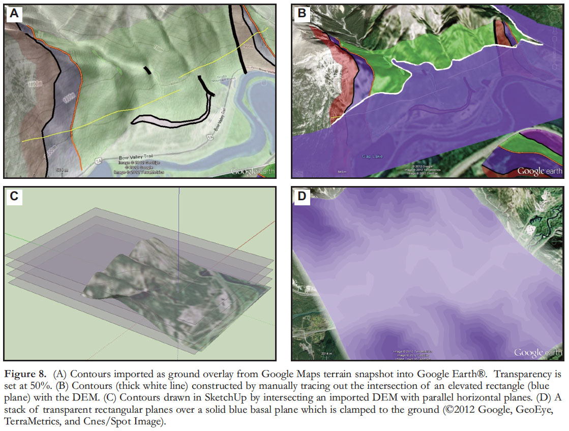
21 Contours are important for map interpretation and are built into Google Maps but strangely not into Google Earth®. We devised four methods for adding contours to the Google Earth® terrain.
22 In the first method (Fig. 8A) a screen shot of the region of interest is taken in Google Maps with its terrain feature switched on. This is imported into Google Earth® as a ground overlay and draped over the matching topography. This works well because Google Maps and Google Earth® share the same DEM (if a map from a different source were draped onto the Google Earth® terrain, the resultant contour lines might be far from horizontal). A disadvantage of this method is that paths or polygons drawn with Google Earth® tools will be covered by the ground overlay image (paths and polygons cannot be given a higher KML draw order). However, if the transparency of the image is adjusted, map features beneath become visible. This approach is the fastest and it produces acceptable visual results if the region of interest is not too large – on the order of 10 km 2 – otherwise, the contours become too dense and the image file becomes very large.
 Display large image of Figure 8
23 The second method (Fig. 8B) involves manually tracing the contours using the Google Earth® ‘Add Path’ tool. Here, the first step is to create a rectangular polygon similar in size to the region of interest. When the altitude mode of this rectangle is set to ‘absolute’ (the height is 1800 m in Fig. 8B) the contact with topography can be seen (indicated with the white bold line) and traced out by hand. This process is then repeated for all the desired altitudes.
24 For the third method, the DEM from Google Earth® is imported into SketchUp using its ‘Get Current View’ tool (Fig. 8C). Once the DEM is imported, by intersecting it with a set of equally spaced horizontal planes, contours can be produced and exported back into Google Earth® as a 3-D model. Two disadvantages of this approach include the limit of ~4 km2 for the area that can be imported and the large file size.
25 The fourth method (Fig. 8D) is a derivative of the second method. Instead of tracing the intersection of the rectangular polygons with the DEM, the rectangles are made 90% transparent (10% opaque) and stacked by copying them while increasing their altitudes. Then a solid colour base rectangle is clamped to the ground under this stack. Here the base colour is blue and the altitude ascends from blue toward white because the base layer is covered with more rectangular planes at each elevation. This method can be completed fairly quickly and can extend over large regions (subject to the effect of Earth’s curvature).
Opportunities Provided by COLLADA Modelling
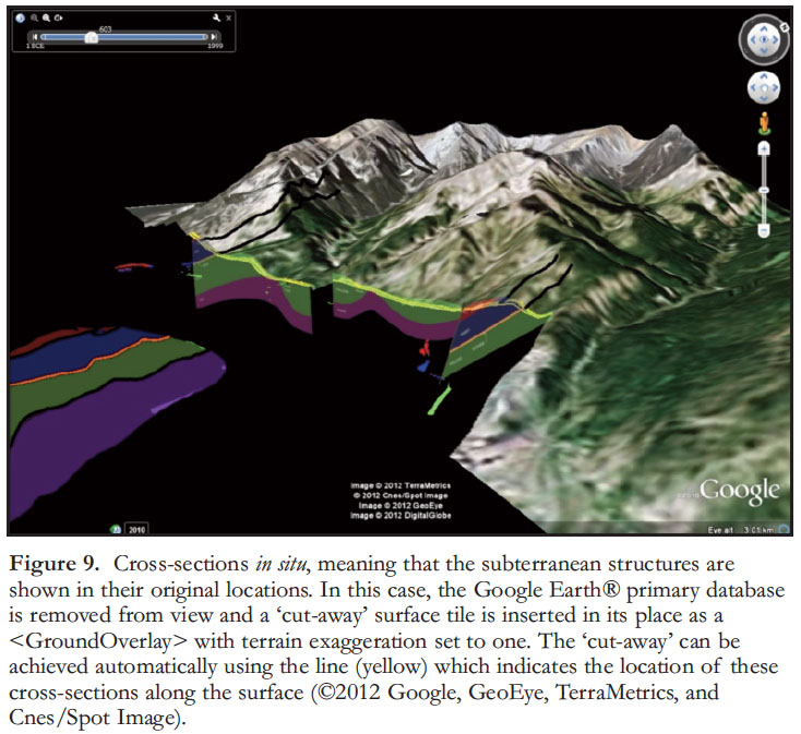
26 The above discussion demonstrates the potential for Google Earth® to be used for visualizing complex geologic structures and processes. Additional steps can be taken to show underground geologic structures in situ (meaning in their original locations) as shown in Figure 9. These KML objects were created using image processing tools to 1) capture a surface image tile, and 2) remove sections of that tile which would obstruct the user’s view of the cross-sections. In version 5 of the Google Earth® desktop application, surface tiles are made transparent by highlighting ‘Primary Database’ in the Layers sidebar and then moving the transparency slider all the way to the left (see ‘A’ in Figure 10). In Google Earth® version 6.2, the primary database is always opaque; instead the Radar item in the Weather Layer must be made transparent. The cut-away tile is reinserted as a ground overlay and is draped on the terrain. An obvious next step would use the line drawn along the surface (the yellow line in Fig. 9) to define the cross-section(s) and perform the surface image tile cut-away. The image tile cut is also a split, where the two resulting sections of the ground overlay can be used to view the cross-sections in situ from opposing directions.
 Display large image of Figure 9
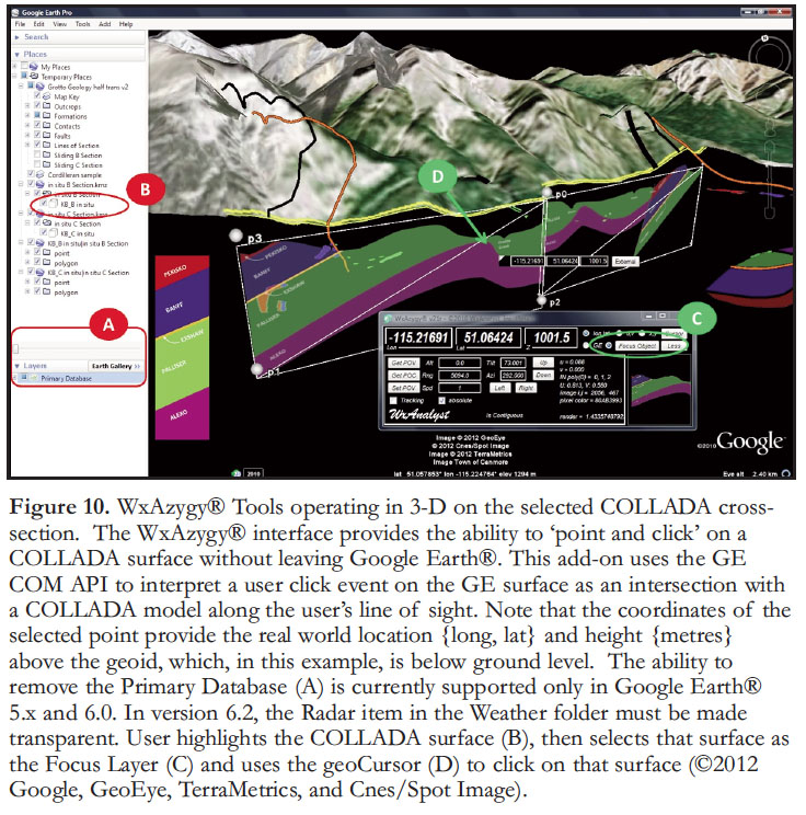
27 Now that the cross-sections have been established in situ, we can apply WxAnalyst’s WxAzygy® Tools to interrogate the cross-sections as shown in Figure 10. This add-on is available (WxAnalyst 2012; Shipley 2012a) for Google Earth® versions running on Microsoft Windows which supports the GE COM API. WxAnalyst’s WxAzygy® Transparent Interface (Shipley et al. 2009, 2010) interprets user mouse clicks on Google Earth® to calculate the corresponding position of that click on a COLLADA surface. The user selects the ‘focus’ COLLADA layer that is to be interrogated then clicks on that COLLADA surface to obtain the coordinates of the point selected on that surface. This method uses the GE COM API to establish the user’s Point Of View (POV) in Google Earth®, so that the resulting coordinates are independent of Google Earth® pan, zoom, rotation, or tilt. The tool also provides a visualization of the COLLADA models using icons and lines which assists the user in identifying the layer that has been selected. The example in Figure 10 shows layer KB_B in situ selected as the Focus Layer with the geoCursor tool in COLLADA triangle [p0,p1,p2]. WxAnalyst’s WxAzygy® interface shows the results of the click in the Southesk/Alexo stratum at a height of 1000 m above the Earth Geoid, which combined with model displacement of 200 m at that location corresponds to a depth of approximately 200 m below the surface. The interface also provides the coordinates of the point on the draped image [i=2056, j=467] and its colour at that point in hexidecimal [A=80h, R=ABh, G=39h, B=93h]. An ‘External’ command is also visible in the cursor for access to additional functions defined by the COLLADA model, as discussed in the WxAzygy® User Manual (WxAnalyst 2010; Shipley 2012b, c, d, e, and f).
 Display large image of Figure 10
28 The WxAzygy® Transparent Interface was developed by WxAnalyst under NASA SBIR Phase 1 funding by the NASA Langley Research Center. Phase 3 funding was subsequently provided by NOAA’s National Climatic Data Center (NCDC) to provide a freeware version of the tools online (WxAnalyst 2012; Shipley 2012a). As of this publication, the GE COM API is available in GE versions 5.x through 6.2 for Microsoft Windows. Google has announced that the GE COM API has been deprecated and may no longer be supported. Additional functions developed beyond the freeware version of the tools include the ability to edit COLLADA models, to draw freehand on COLLADA model surfaces, and to change colours of the images draped on the COLLADA models, with all operations performed in situ without leaving Google Earth® (Shipley 2012a, b, c, d, and e for more detailed user instructions).
DISCUSSION
29 The ultimate goal for future Google Earth® models expanding upon the Grotto Creek model presented here is to create a series of 3-D interactive VFTs through the Canadian Cordillera. As mentioned by Whitmeyer et al. (2010), these interactive Google Earth® geological maps are more intuitive for non-professionals than traditional paper maps and cross-sections. It is also hoped that VFTs employed as a supplemental introduction to real field experiences will greatly decrease the overwhelming nature of first field experiences (as summarized in Mogk, 2011). In the future, this pilot Google Earth® model will be expanded to include the extensive mapping and structural analysis outlined by Clark (1949), Balley et al. (1966), Price (1970), Dahlstrom (1970), Price and Mountjoy (1970), Monger and Price (1979), Price (1994), McMechan (1995), and Simony in Spratt et al. (1995).
30 Google Earth® and SketchUp were used because they are well integrated with each other, supported by multiple platforms, relatively simple to use, widely available, and free. For most geosciences tasks, SketchUp is sufficiently powerful; however it cannot wrap a texture around a sphere or draw a line on a curved surface. There are free Ruby plug-ins available for SketchUp that enable these tasks. Other software is available that could create similar models to the one presented here, such as Gplates from Earthbyte, Layerscape from Microsoft, Move software from Midland Valley, NASA World Wind, GEON, Open Topography, etc. SketchUp was used because the others are either not free, not cross platform, or have a steep learning curve. However, with the sale of SketchUp to Trimble Navigation Inc., the future of free SketchUp is unclear.
31 Custom sliders were created using COLLADA, JavaScript, and Google Earth® APIs. Once again, these were used because they are well integrated, supported by multiple platforms, relatively simple to use, widely available, and free. While there are many other possibilities for creating 3-D models such as LightWave 3-D, Maya, 3ds Max, many of these are heavy weight modelling applications with steep learning curves that would be underused for geoscience modelling.
32 Finally, Google Earth® Layers were adjusted and manipulated using WxAzygy® to create a queryable ’cut-away’ transparent view of in situ geology. One powerful application of WxAzygy® is that it provides a convenient platform for creating COLLADA and KML directly in Google Earth®. Unfortunately, Google Earth® recently announced that it will no longer support the GE COM API, which makes the creation of transparent tiles much more difficult.
CONCLUSIONS
33 Google Earth® and other virtual globes present excellent media for analysis of surface data such as geological maps draped over topography. The addition of Google Earth® API, KML, and COLLADA has greatly enhanced the 3-D visualization capacity for Google Earth® models. COLLADA models retain azimuthal orientations (unlike placemark icons), while KML permits users to add custom data in a variety of formats, and the Google Earth® API combined with JavaScript enables users to manipulate COLLADA model behaviour (De Paor and Whitmeyer 2011).
34 Another significant application for Google Earth® models is the ability to immediately ‘fly and explore’ features embedded within the text of papers such as this. Regardless of the potential for assisting students in acquiring the necessary spatial cognitive skills during their voyage from novice student to professional geologist, most people are engaged by this incredible technology.
35 Further Google Earth® applications introduced here include the use of vertical sliders to create emergent cross-sections capable of sliding through topography, horizontal sliders that reconstruct a structural reconstruction model, and queryable ‘cut-away’ cross-sections embedded into topography.
ACKNOWLEDGEMENTS
36 This paper is dedicated to the memory of Dr. Cynthia Riediger. The Jura Creek Exshaw Formation type locality outcrop was informally named ‘Cindy’s outcrop’ during the MRU field school 2010. Amanda Taylor’s digitizing of the cross-sections for the structural reconstruction model was greatly appreciated as is her input on potential educational applications of these Google Earth® models. In addition to Jonathan Fell, the numerous field school students at Mount Royal University and the University of Calgary have been instrumental in illustrating the need for Google Earth® models such as presented here to augment their educational experience.
37 The custom slider construction was partially supported by NSF TUES 1022755, NSF GEO 1034643, and a 2010 Google Faculty Research Award supporting Dordevic. Any opinions, findings, and conclusions or recommendations expressed in this paper are those of the authors and do not necessarily reflect the views of the National Science Foundation or Google Inc.
38 WxAnalyst’s WxAzygy® Transparent Interface was developed in part under NASA SBIR Phase I Contract NNX09CF28P and NOAA National Climatic Data Center SBIR Phase III funding under Contract NEEF4100-10-18847. WxAzygy® is a registered trademark of WxAnalyst, Ltd.
39 The manuscript benefitted greatly from reviews by Glen Stockmal and Fraser Keppie. This paper would not have been possible without the greatly appreciated coordination and editorial support of Declan De Paor.