Series
Remote Predictive Mapping 3.
Optical Remote Sensing – A Review for Remote Predictive Geological Mapping in Northern Canada
SUMMARY
Optical remotely sensed data have broad application for geological mapping in Canada’s North. Diverse remote sensors and digital image processing techniques have specific mapping functions, as demonstrated by numerous examples and associated interpretations. Moderate resolution optical sensors are useful for discriminating rock types, whereas sensors that offer increased spectral resolution (i.e. hyperspectral sensors) allow the geologist to identify certain rock types (mainly different types of carbonates, Fe-bearing rocks, sulphates and hydroxyl-(clay-) bearing rocks) as opposed to merely discriminating between them. Increased spatial resolution and the ability to visualize the earth’s surface in stereo are now offered by a host of optical sensors. However, the usefulness of optical remote sensing for geological mapping is highly dependent on the geologic, surficial and biophysical environment, and bedrock predictive mapping is most successful in areas not obscured by thick drift and vegetation/lichen cover, which is typical of environments proximal to coasts. In general, predictive mapping of surficial materials has fewer restrictions. Optical imagery can be enhanced in a variety of ways and fused with other geo-science datasets to produce imagery that can be visually interpreted in a GIS environment. Computer processing techniques are useful for undertaking more quantitative analyses of imagery for mapping bedrock, surficial materials and geomorphic or glacial features.
SOMMAIRE
Les données recueillies par télédétection optique offrent beaucoup de possibilités pour la cartographie géologique des régions nordiques canadiennes. La diversité des télécapteurs et des techniques de traitement numérique des données permet la définition de fonctions de cartographie spécifique, tel que l’illustre de nombreux exemples et interprétations associées. Des capteurs optiques de moyenne résolution sont utiles pour différencier les types de roche, alors que les capteurs à plus fines résolutions (les capteurs hyperspectraux, par ex.) permettent au géologue de subdiviser certains types de roches (principalement différents types de carbonates, roches ferrugineuses, roches à sulfates et à hydroxyle (argile). Une meilleure résolution spatiale et la fonction de vision stéréoscopique sont maintenant offertes sur une gamme de capteurs optiques. Cela dit, l’utilité de la télédétection optique pour la cartographie géologique est fortement tributaire des conditions de la géologie de surface et de son environnement biophysique, le potentiel prédictif de la télécartographie étant maximal pour les régions exemptes d’une couverture épaisse de dépôts glaciaires ou d’une couverture végétale/lichen caractéristique typique des environnements longeant les côtes. Divers procédés permettent de rehausser l’imagerie optique et de réaliser des fusions avec d’autres jeux de données géoscientifiques et de produire une imagerie visuellement inter-prétable en environnement de SIG. Les techniques de traitement de données par ordinateur sont utiles pour d’autres types d’analyse quantitative d’imagerie pour la cartographie des matériaux de couverture du socle et pour répertorier des formes glaciaires et géomorphologiques.
INTRODUCTION
1 Canada needs efficient methods for upgrading its geoscience knowledge base because of its vast territory and world-class mineral potential. This is primarily achieved by updating and completing the national geological map coverage; however, many areas in Canada’s north are inadequately mapped from both a bedrock and a surficial materials perspective. In the past, the coverage and publication of traditional geological paper maps was a process spanning decades and requiring years of associated fieldwork. Today, the need to attract investment in the mineral resource industry requires an alternative, more time-efficient approach to geological mapping. As a result, techniques of Remote Predictive Mapping (RPM) have, in recent years, been tested in pilot projects carried out by Canadian national and provincial geological surveys. Basically, RPM is an integrated geological mapping approach, in which existing datasets are re-compiled by interpreting aerial photographs, satellite imagery and airborne geophysical data, all in a digital environment. This, in combination with strategically planned field follow-ups, allows for the production of up-to-date digital geological map databases, over large regions, more frequently (two to three years). The digital standardized format of such modern archives also provides geological information in a structured form that facilitates future updates. Generally, RPM provides focus for regional mapping and exploration efforts as well as first-order geological information in areas hat are poorly mapped. A more detailed presentation on RPM is provided by Schetselaar et al. (2007) and Harris (2008).
2 Optical remote sensing can play a significant role in the RPM process as many optical sensors offering high-quality data are presently available to the geologist. Much spectral information on specific rocks and minerals that can aid in geological mapping and provide information on geological structures and surficial materials can commonly be acquired by optical remote sensing. This paper provides a review of optical remote sensing for the mapping geologist and provides general discussions on theoretical principles, sensors and processing techniques, using examples from Canada’s North.
THEORETICAL PRINCIPLES
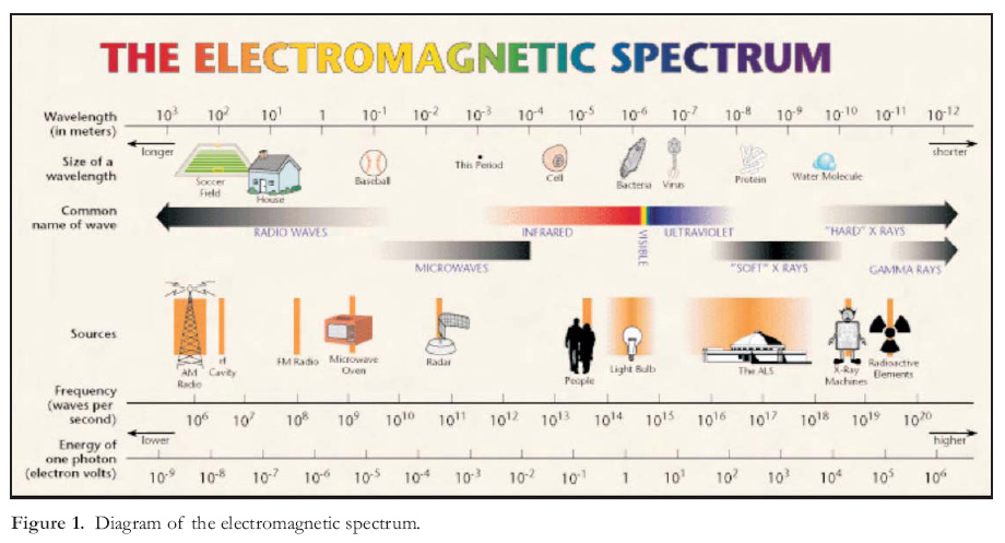
3 Optical remote sensing is based on creating an image using reflected solar energy from selected intervals of the electromagnetic (EM) spectrum; these intervals range in wavelength from 0.4 to 3.0 microns (μm) and include the visible (V), near infrared (NIR) and short wave (or middle) infrared (SWIR). The visible, and near infrared, are commonly collectively referred to as VNIR (Fig. 1). The sun is the source of energy for optical remote sensing; hence optical sensors (e.g. LANDSAT) are passive, as no energy is generated by the sensor in the data-acquisition process. Data generated are readily available in a digital raster or grid format in which individual image elements called pixels contain a digital number (DN) that is proportional to the amount of solar energy reflected at a given wavelength. Remote sensing can also be conducted in the thermal infrared portion (TIR) of the EM spectrum; this involves the sensing of emitted (as opposed to reflected) energy (heat) from the Earth at wavelengths from 3 to 5 μm and 8 to 14 μm. Thermal remote sensing does offer advantages for geological mapping of certain minerals, but is not discussed in this review paper.
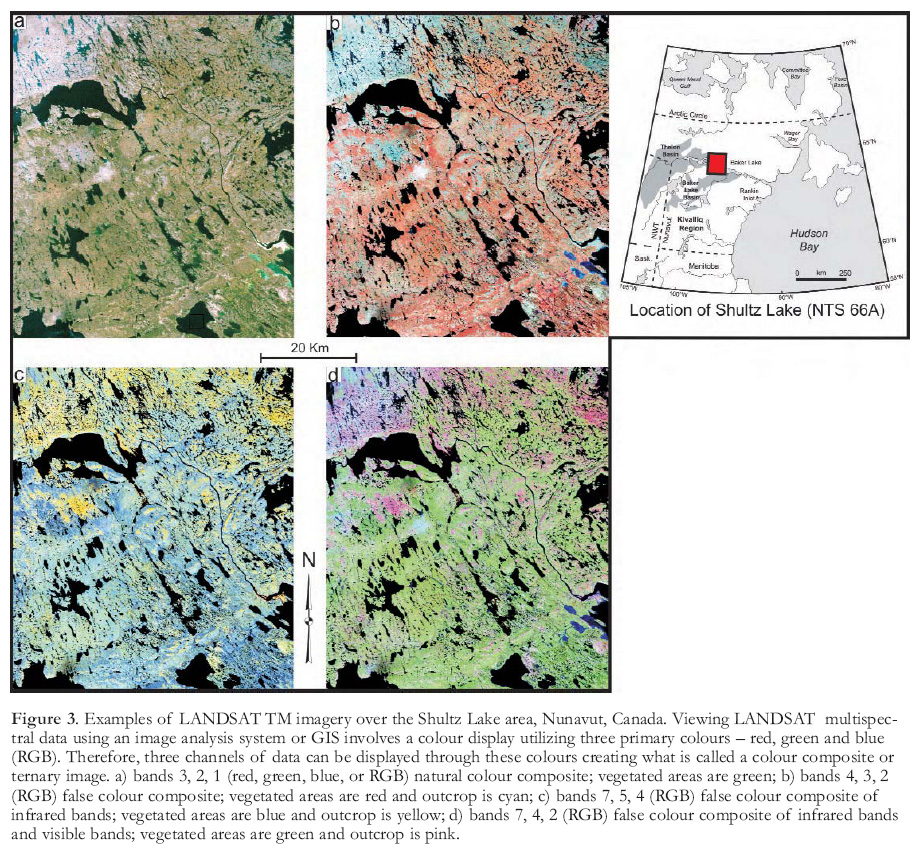
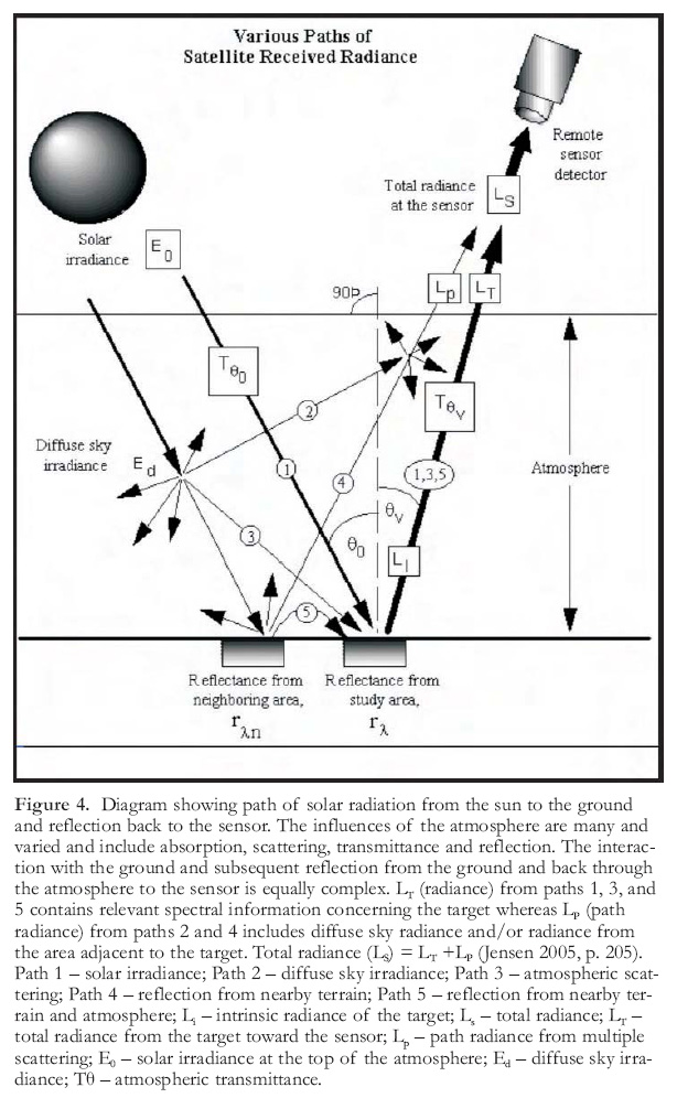
4 Optical sensors are further characterized by a series of bands (or channels) (Table 1), each providing a separate image that can be viewed and interpreted separately (Fig. 2), or combined as red–green–blue (RGB) ternary images (Fig. 3), in which colour variations are created by the combination of three channels. A unique image, in which different terrain and surficial features are enhanced, will result for each band, as the incoming solar energy will interact differently with the atmosphere and with the earth’s surface (Fig. 4), depending on the wavelength.
 Display large image of Table 1
5 Overall, the resolving capability of a sensor is a combination of spectral coverage, spectral resolution, spatial resolution and signal-to-noise ratio. These characteristics of a sensor (both airborne and satellite-borne) are fixed and cannot be altered post-sensor construction. Optical sensors are typically classified as multispectral or hyperspectral. Multispectral sensors have a limited number of bands (generally less than 30), of wider bandwidth (100 nanometres (nm) or more), whereas hyperspectral sensors are characterized by many bands (30 to 100s) of very narrow bandwidth (3 to 20 nm).
6 The number of wavelengths covered and the bandwidth (i.e. width of the channel in μm or nm) dictates the spectral resolution of the sensor. Higher spectral resolution increases the probability of unequivocally identifying various earth materials (such as specific minerals or groups of minerals defining a particular lithotype) as opposed to simply discriminating materials or mineral groups. More channels or increased spectral resolution increases the application of the optical sensor, as different parts of the EM spectrum are more suited for discriminating different minerals. For example, the VNIR is particularly good at discriminating various iron-bearing minerals whereas clays and carbonates are better discriminated in the SWIR (Fig. 5). Recently, much emphasis has been placed on hyperspectral remote sensing, which simply refers to an optical sensor with many channels. LANDSAT, for example, has 6 channels in the VNIR and SWIR, whereas a hyperspectral optical sensor, such as the airborne PROBE system has 128 channels, and the airborne AVRIS sensor has 256 channels in same segment of the EM spectrum (see Table 2 for a summary of selected optical sensors).
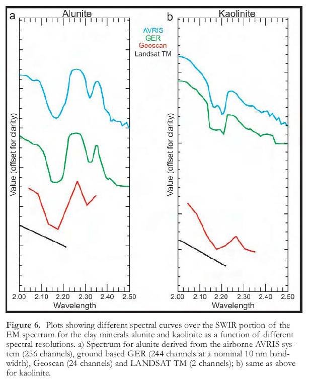
7 Optical sensors exploit the variable reflectance of earth features that result from differences in surface chemistry. Interaction of the incoming energy with the surface is controlled by processes at the molecular level (e.g. vibrations, oscillations of molecules), which determines whether the energy is absorbed, reflected or transmitted, resulting in a unique spectral signature for the particular target. The importance of spectral resolution can be clearly seen on spectral plots (Fig. 6) for two clay minerals (alunite and kaolinite) recorded by sensors with different spectral resolutions and by ground-based spectrometers. Alunite and kaolinite can be uniquely identified by their spectral characteristics (position and shape of absorption troughs between 2.1 and 2.2 μm) using the AVRIS and GER sensors, which have sufficient spectral resolution to resolve their spectral properties. However, because LANDSAT is characterized by low spectral resolution (only 2 bands in the SWIR), alunite and kaolinite may be discriminated but cannot be uniquely identified or separated.
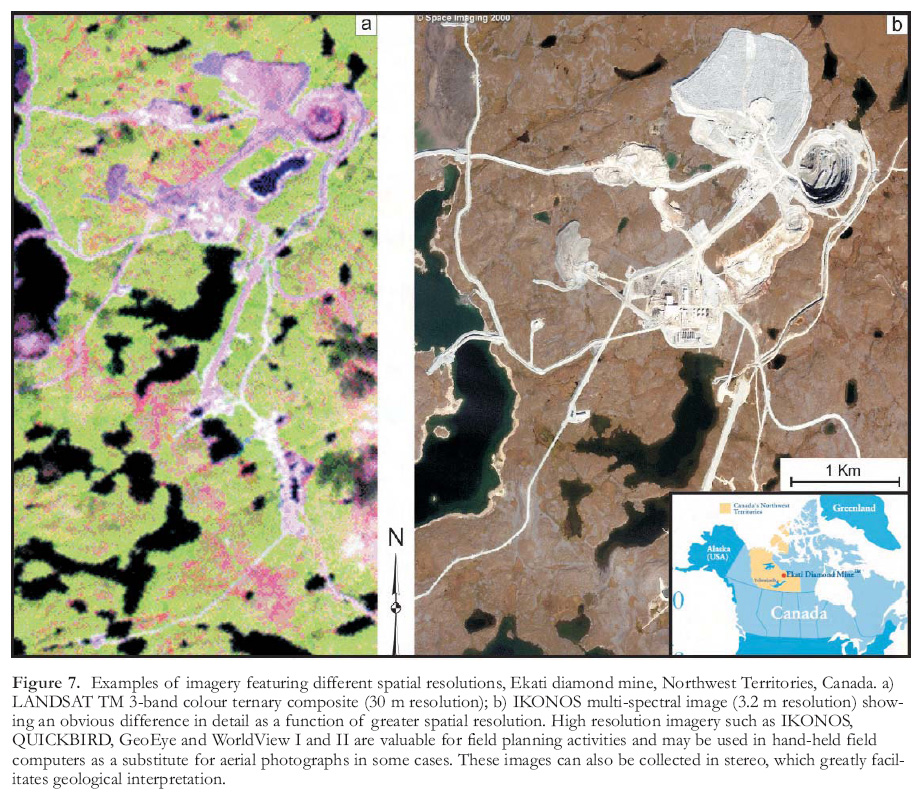
8 Another important consideration is spatial resolution, which for optical sensors is defined by the flying height and instantaneous field of view. The amount of geological information that can be extracted from an image is strongly dependent on the spatial resolution of the sensor (Fig. 7). Moderate resolution sensors such as LANDSAT (30 m resolution for multispectral bands, and 15 m resolution for panchromatic bands) are useful for regional mapping campaigns (>1:50 000 scale) and can offer information on lithology, structure and infrastructure for field planning purposes. Higher resolution sensing is currently offered by satellite-borne sensors such as ASTER, IRS and SPOT-5. Paralleling the recent development of optical sensors offering higher spectral resolution (i.e. hyperspectral) are sensors that now offer metre to sub-metre spatial resolution from space (e.g. IKONOS, QUICKBIRD, GEOEYE, WORLD-VIEW –Table 2). This imagery, although expensive to purchase, rivals aerial photography and often exceeds aerial photographs in terms of spatial resolution and the amount of terrain detail that can be interpreted, as many of these sensors offer multispectral capabilities. This type of high spatial resolution imagery is very useful for not only detailed mapping but also for logistical planning activities. Additionally, many of these sensors can collect stereo imagery. Many examples of high resolution sensors and moderate resolution sensors can be found in Google Earth and Microsoft Virtual Earth.
 Display large image of Figure 2
9 Another feature of a sensor is its dynamic range, or signal-to-noise ratio, which is the amplitude of the signal relative to the amplitude of the noise of the sensor. The higher the signal-to-noise (S/N) the better a signal can be resolved and identified. It is often advantageous to process the data using the full dynamic range as opposed to compressing the data (e.g. from 32 or 16 to 8 bits), as this represents a loss of potentially useful information.
10 Optical remote sensors record reflected solar energy; hence there is a need to deal with complicating factors such as the atmosphere (Fig. 4), which can seriously degrade image quality. Obviously, imaging is not possible in cloudy conditions, but even in apparent cloud-free conditions the effects of the atmosphere (e.g. scattering, absorption) must be taken into account in the imaging process. Atmospheric corrections often must be applied to quantitatively interpret the data. This is especially true for optical remote sensing in northern latitudes, where the effects of the atmosphere are compounded by low sun (illumination) angles, which can have a serious effect on the quality (low S/N) of the resulting data. The path that solar energy takes from source (sun) to destination (sensor) is complex (Fig. 4), and many variables can have a profound effect on the resulting imagery. These effects must be accounted for (corrected) in the final image product, especially for hyperspectral sensors.
 Display large image of Figure 3
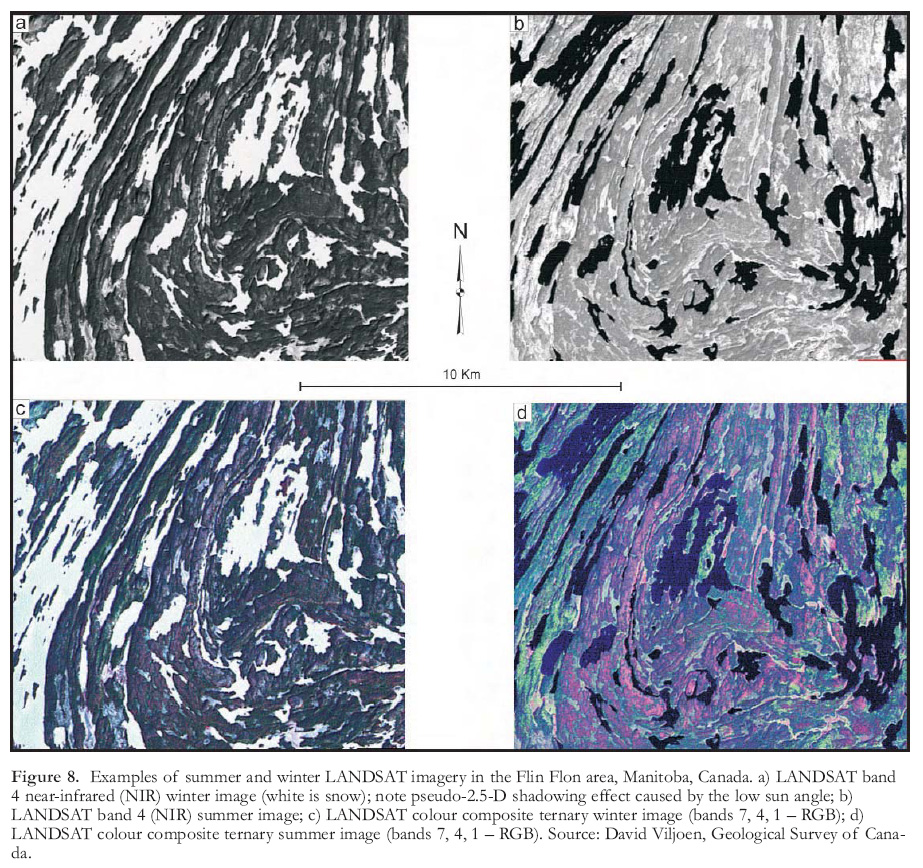
11 It must be stressed that optical remote sensing only collects information on the surface of the earth, unlike magnetic remote sensing, for example. As mentioned above, cloud cover will completely reflect and/or absorb incoming solar radiation, so this is a limiting factor for remote sensing in Canada’s north. However, when complete coverage of a study area is obtained, the resulting imagery will normally suffice for future mapping programs, as the objects of interest (i.e. geology, terrain) do not change significantly over time. Nevertheless, the season in which the optical data are acquired will make a significant difference in the way a given area will appear, because of seasonal climate variations (e.g. snow vs. no snow, fall senescence etc.) as well as acquisition geometries (sun angle). Imagery acquired during winter looks appreciably different than imagery collected in the same area during the summer (Fig. 8). Lower winter sun angles often produce imagery that is optimal for mapping geological structures and glacial and geomorphologic features because of the pseudo 2.5-D shadowing effect (Fig. 8a, c). Therefore, the season of acquisition is as important as spectral and spatial resolution for geological mapping applications.
12 In addition to the system factors, discussed above, the most important terrain factors that should be considered when using optical imagery for structural, lithological and surficial mapping include:
- The nature and age of the bedrock;
- The type and amount of surficial cover (which defines the target for surficial mapping but is an impediment to bedrock mapping);
- The biophysical environment, such as the type and amount of vegetation (including lichen) and snow cover; and
- The topography.
12 Lichen can be a particularly strong impediment to bedrock mapping using hyperspectral remote sensing even in areas with abundant outcrop, as lichen can mask the diagnostic spectral signatures of the rocks and minerals beneath (Bechtel et al. 2002).
 Display large image of Figure 4
13 Optical remote sensing, like any form of remote sensing (including geophysics), is not an all-encompassing tool or solution for geological mapping, and the success of the specific geological application is dependant on both the system and the terrain factors discussed above. Obviously, optical remote sensing will be more successful for lithological mapping in terrain with good bedrock exposure and less surficial and vegetation cover, whereas surficial mapping using optical imagery has fewer geographic, terrain and biophysical restrictions.
DATA
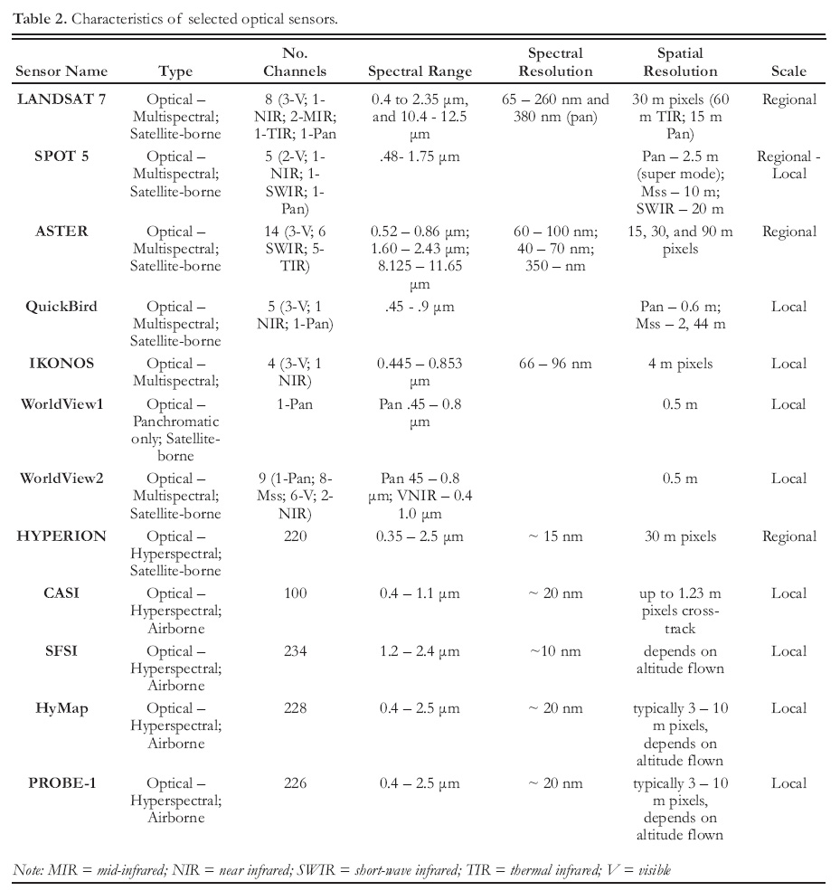
14 A variety of optical sensors is available for geological mapping, and a summary of the characteristics of selected instruments is provided in Table 2. Sensors are often broadly characterized by their host platform; i.e. whether they are satellite-borne or aircraft-borne. Satellite-borne sensors have the advantage of providing synoptic coverage from a stable platform, as there is no atmosphere to affect the motion of the sensor. They are expensive to build and deploy in lower earth orbits, but once in orbit they have a lifespan of many years and the costs of data acquisition per scene are generally low. However, satellite-borne sensors are limited in other ways. Given that the orbit is fixed, and the pointing direction is not generally adjustable, optical sensors are very dependent on good weather for successful data acquisition. In some areas of the world (e.g. the tropics and northern regions), this is a considerable problem because of almost perpetual cloud cover. Furthermore, in recent years newer optical sensors are being mounted on smaller satellites because of cost considerations; hence, they have payload limitations that may limit data storage, leading to limitations on data scene size and spatial resolution. HYPERION, one of the few satellite-borne hyper-spectral sensors presently in orbit, has limited spatial resolution (30 m) and serious problems with S/N. Generally, for satellite-borne sensors there is a trade-off between high spatial and high spectral resolution. For example, the IKONOS satellites have a spatial resolution of 4 m for 4 channels of data; in contrast, the ASTER satellite-borne sensor has 14 available channels but a spatial resolution of only 15 to 90 m. Stereo coverage from many optical sensors (SPOT, ASTER, GeoEye, IKONOS, QuickBird, WorldView 1 and 2) is also possible because different view angles produce parallax differences in stereo pairs. These stereo images can be viewed through stereoscopes or directly on a computer screen by using special stereo glasses. This greatly facilitates the geological interpretation process.
 Display large image of Figure 5
15 Airborne sensors are typically mounted on small aircraft and engaged for project or site-specific acquisitions. Hence, the cost per scene is much higher, and costs will vary across the globe because of varying mobilization/demobilization costs. Aircraft generally fly close to the surface of the earth (less than 10 km), hence airborne data are often characterized by much better spatial resolution (3 to 10 m pixels or less); however, this is changing rapidly with the advent of a new generation of satellite-borne sensors that have extremely high spatial resolution. Acquisition of data from hyperspectral sensors having broad spectral coverage (e.g. VNIR + SWIR) and high spatial and spectral resolution is, therefore, possible with airborne platforms. The biggest challenge with airborne hyper-spectral data is correcting and processing the large volume of data generated.
Error Correction and Registration
16 Raw, remotely sensed optical data (Level 0), once collected, is typically corrected to Level 1 data, which accommodates known radiometric and geometric errors. These data are generally delivered as a ‘path’ image, which is an image that is orthogonal to the path over which it was collected, but has not been adjusted to represent its true position over the surface of the earth (georectification). A number of Level 1 subtypes exist, and vary depending on the sensor. For example, ASTER L1A data has the Level 0 to Level 1 corrections calculated, but they are only appended, not applied, whereas for ASTER L1B data, the corrections have been applied. For LAND-SAT imagery, various data products are available, including L1G, in which the data are orthorectified using a simple Geotopo global Digital Elevation Model (DEM). Typically, such labelling is employed more for imagery acquired from satellite-borne sensors; variations in terminology may also be encountered.
17 Post-processing of the data past Level 1 is often required, depending on the sensor and the application of the data. Most sensors, even commercial ones (e.g. IKONOS, QUICK-BIRD), deliver a product formatted with digital numbers (DN). For non-quantitative applications the data could be used directly, but in most cases it is preferable to convert digital numbers using the following corrections:
- Gains and offsets or unit conversion coefficients are applied to convert the data from digital number (DN) to radiance (W/m 2/sr/µm: Watts/square metre/steradian/specific frequency in hertz);
- Atmospheric corrections to convert the data from radiance to relative reflectance or at-surface reflectance.
18 For some sensors, particularly those that are categorized as ‘research sensors’ (e.g. ASTER, HYPERION), many other corrections are necessary to address errors inherent in the instruments. For most applications, only major sources of instrument error will require correction, whereas for others more precise correction will be required. Most hyperspectral datasets will require accurate atmospheric correction, as the data are often used to generate precise spectral signatures of various Earth features.
 Display large image of Figure 6
19 A number of commercial software products are available for precise and detailed atmospheric correction, including ACORN and FLAASH. These are more widely applied to hyperspectral data, but may also be used for multispectral data (e.g. ASTER). Simpler correction techniques than those employed by the above packages include Internal Average Relative Reflectance, Flat Field Calibration, and Empirical Line Correction. These simpler techniques, which generate relative, as opposed to absolute reflectances, are often appropriate for multispectral sensors. A comprehensive summary of atmospheric correction methods is provided by the United States Geological Survey (USGS 2003).
SELECTED OPTICAL SENSORS USEFUL FOR RPM
20 A wide range of optical sensors is available for use, and for the inexperienced user it can be a daunting task choosing the sensor that is most appropriate for a given geological application. Hence, Table 2 presents a summary of the sensors best suited to RPM applications.
High Spatial Resolution Satellite-borne Sensors
21 IKONOS is a commercial satellite that was deployed in a sun-synchronous orbit (651 km) in 1999 by Space Imaging (now owned by GeoEye). It has two sensors featuring extremely high spatial resolution: a 403 nm panchromatic band sensor having 1 m resolution, and a multispectral sensor with 4 bands (MS-1 to MS-4 at blue, green, red and near infrared) at 4 m resolution (at 26° off-nadir; slightly better resolution at nadir). Images can be ordered from either telescope, or both, and combinations of products are also available including orthorectified products.
22 QUICKBIRD is also commercially operated, and was launched by Digital Globe in 2001. It is in a synchronous orbit, slightly lower in altitude than IKONOS (450 km), with a 3 to 7 day revisit cycle. It has two sensors, similar to IKONOS, but has slightly higher spatial resolution. The 550 nm panchromatic band sensor provides imagery with a spatial resolution of 0.61 m (at nadir), and the 4 band multispectral sensor (blue, green, red and near infrared) provides 2.44 m resolution (also at nadir). As with IKONOS, a variety of different image products is available.
23 The strength of IKONOS and QUICKBIRD lies in their ability to generate high-quality, high-resolution imagery that can, to some degree, replace the use of aerial photographs. IKONOS has an image swath of 11.3 km (nadir), and 13.8 km (26° off-nadir), whereas QUICKBIRD has a slightly larger image swath of 16.5 km (nadir). IKONOS and QUICKBIRD images are particularly useful for initial site surveys and field work planning and mapping. Although the imagery from both satellites is of very high quality, it is quite expensive: acquisition of a new scene costs more than $3K. A more cost-effective solution is to order previously imaged scenes contained in the data archive for each instrument, at a cost of ~ $1K or less.
24 GeoEye, launched in September 2008, acquires panchromatic data at a spatial resolution of 0.41 m and multispectral data at a resolution of 1.65 m. Both image types can be collected in stereo. A global repeat cycle of 3 days allows collection of over 350 000 km 2 of pan-sharpened imagery on a daily basis. Digital Globe’s World-View 1 satellite launched in 2007 offers high quality panchromatic imagery at a resolution of 0.5 m with a repeat cycle of 1.7 days, allowing for the collection of up to 750 000 km 2 of imagery per day. Worldview 2 offers both panchromatic imagery and multispectral imagery in the VNIR range at a spatial resolution of 0.5 m.
 Display large image of Figure 7
25 The SPOT series of satellites has been operational since 1986 and comprises four satellites culminating in SPOT-5, launched in May 2002. The sensors’ oblique viewing capability (i.e. a steerable beam) offers frequent imaging of a given geographic area as well as stereoscopic viewing. SPOT-5 comprises two panchromatic channels characterized by 5 m spatial resolution, three channels in the VNIR with 10 m pixels, and one SWIR channel with a 20 m pixel (Table 2). The two panchromatic channels can be combined to generate a 2.5 m-resolution product (super-mode) that is ideal for mapping and logistical applications. The super pan-mode can be used as a replacement for aerial photographs because it has sufficiently high spatial resolution and is affordable for use in hand-held mapping devices. This imagery has been used successfully by the Geological Survey of Canada for a number of regional mapping projects.
Moderate Spatial Resolution Satellite-borne Sensors
26 LANDSAT 7 ETM+ is the latest in a series of LANDSAT satellites (LAND-SAT 1 to 5 and 7) deployed by the US Government, in conjunction with NASA, the US Geological Survey and the Jet Propulsion Laboratory. The still-operational LANDSAT 5 was followed by LANDSAT 7, which was deployed in April 1999 in a sun-synchronous orbit at an altitude of 705 km. It has a repeat cycle of 16 days, and a nominal equatorial crossing of approximately 10 am local time (i.e. at the location where the crossing occurs).
27 LANDSAT 7 has an advanced version of the Thematic Mapper (TM) sensor that was deployed on LAND-SAT 5, called Enhanced Thematic Mapper Plus (ETM+). The ETM+ sensor comprises three different telescopes, covering a wide range of the EM spectrum. There are four channels in the VNIR (1 to 4; blue, green, red and near infrared), two channels in the SWIR (5 and 7), one channel in the thermal infrared (TIR; channel 6, with data available at low and high gain), and one panchromatic channel (8). Channel 8 has a spatial resolution of 15 m, channels 1 to 5 and 7 have a spatial resolution of 30 m, and the thermal channel (6) has a spatial resolution of 60 m.
 Display large image of Figure 8
28 The LANDSAT series of satellites provided the first global, optical multispectral imagery suitable for geological applications, and has been instrumental in introducing remote sensing as an exploration and mapping tool to the geological community world-wide. The next generation of LANDSAT satellites (LANDSAT 8), termed the LANDSAT Data Continuity Mission, has a planned launch sometime in 2011.
29 The ASTER sensor is one of five different sensors installed on the Terra Satellite, which was produced and launched by a joint venture (TERRA) involving the US Government (NASA), and the Japanese Government’s Ministry of Economy Trade and Industry. ASTER is the flagship sensor on TERRA (the others being CERES, MERIS, MODIS, and MOPPET), and was designed as the first stage of a series of new Earth Observation Satellites (EOS) by the US and International partners. TERRA was launched into a sun-synchronous orbit at Vandenburg Air Force Base in December 1999, and first started acquiring data on February 24, 2000. TERRA has a 16-day repeat cycle, and an equatorial crossing at approximately 10:30 am local time.
30 The main objective of ASTER is to assist in improving the understanding of local- and regional-scale processes on, or near, the Earth’s surface and lower atmosphere. ASTER is a multispectral sensor with a total of 14 channels acquired by four individual telescopes. There are three channels in the VNIR (1, 2, 3N), a second, back-looking telescope with a single band in the VNIR (3B), six channels in the SWIR (4, 5, 6, 7, 8, 9), and five channels in the TIR (10, 11, 12, 13, 14). Note that the VNIR does not have the blue band found in LANDSAT. The VNIR telescopes have a spatial resolution of 15 m, slightly better than LANDSAT’s 30 m, and the SWIR and TIR have a spatial resolution of 30 and 90 m, respectively. Although ASTER has limited spatial and spectral resolution when compared to a hyperspectral sensor, it clearly provides an opportunity to carry out spectral mapping on a regional scale (e.g. 1:250 000), and has been shown in some applications to provide good results at scales of 1:50 000 or larger (Cudahy 2002; Oliver and van der Wielen 2006).
31 ASTER has also been evaluated directly as a tool for RPM, with successful results (Wickert et al. 2005). It is a very useful sensor for RPM as it offers an increased number of channels of narrower bandwidth in the SWIR and TIR compared to LAND-SAT (Table 2), hence it has an increased multispectral mapping capability. The narrower bandwidth makes it possible to resolve spectral responses in the SWIR that are grouped into two broad bands in LANDSAT. Thus, ASTER can distinguish different mineral groups (e.g. different groups of clays) that may be associated with specific lithotypes or alteration zones characteristic of certain types of mineral deposits. Although ASTER falls far short of the capability of hyper-spectral sensors in its ability to differentiate mineral species (Fig. 6), the global availability of ASTER as a satellite-borne platform and its low cost as a research level satellite (US $80/scene) makes it an excellent exploration and mapping tool for geological applications. Further details on the use of ASTER for geological mapping can be found in Wickert et al. (2005).
Hyperspectral Satellite-borne Sensors
32 HYPERION, the first publicly available satellite-borne hyperspectral sensor, was launched by the USGS in 2000. It was built as a satellite version of the airborne TRWIS sensor. HYPERION is a ‘pushbroom’ hyper-spectral sensor that has 220 channels ranging from 0.35 to 2.5 µm; it has very narrow band-widths (10 nm), and a spatial resolution of 30 m (note: a ‘pushbroom’ sensor comprises a line of sensors arranged perpendicular to the flight direction of the satellite). HYPERION consists of two spectrometers, one for the VNIR (357–1055 nm), and the second for the SWIR (851–2576 nm). Of the 220 channels, only 180 can be used, because of spectral overlap and mis-alignment or missing data. Overall, the narrow bandwidth provides for excellent spectral resolution, providing the capability to discriminate between different minerals spectrally, even though the pixel size is the same as LAND-SAT (30 m). With its increased channels and associated high spectral resolution, this sensor is a major technological step-up from multispectral sensors, as the sensor is capable of mapping mineral end members.
33 Unfortunately, HYPERION has a very low S/N relative to that of a typical airborne sensor such as HyMap. The S/N for HYPERION is on the order of 50:1, and is particularly low over the SWIR part of the EM spectrum. This contrasts with a reported S/N for HyMap of >500:1. This means that more subtle spectral absorption features will be more difficult to differentiate in HYPERION data, and that good illumination conditions (little to no cloud, high sun angle) are of particular importance for the acquisition of this imagery.
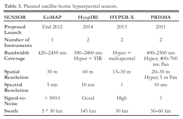
34 Over the next 5 to 10 years, several countries have plans for the development and launch of satellite-borne hyperspectral sensors (Table 3). This will obviously be beneficial for the spectral differentiation of rock types and minerals; however, spatial resolution may be a limiting factor for very detailed (mine-scale) geological studies.
Hyperspectral Airborne Sensors
35 Several airborne hyperspectral sensors (Table 2) have provided limited coverage of the Canadian landmass. Areas for which hyperspectral data have been acquired include parts of Baffin Island (available through the Geological Survey of Canada and the Canada Centre of Remote Sensing – CCRS) and the Sudbury Basin in Ontario (available through CCRS).
36 The SFSI sensor is a grating-based, ‘pushbroom’ imaging spectrometer. It has 234 channels that cover the 1219–2437 nm range, an average spectral sampling interval of 5.2 nm, and a nominal bandwidth of 10 nm (Neville et al. 2003). The CASI sensor acquires data from up to 228 spectral channels in the 400–1000 nm range. The AVRIS sensor is operated by NASA’s Jet Propulsion Laboratory and collects 224 channels between 400 and 2500 nm. The PROBE sensor developed by Earth Search Sciences Inc. collects 128 channels in the 400–2500 nm range; the PROBE-1 can be flown over various altitudes, providing spatial resolution of 1 to 10 m and swath widths from 1 to 6 km.
DATA INTERPRETATION FOR GEOLOGICAL APPLICATIONS
Bedrock Structure
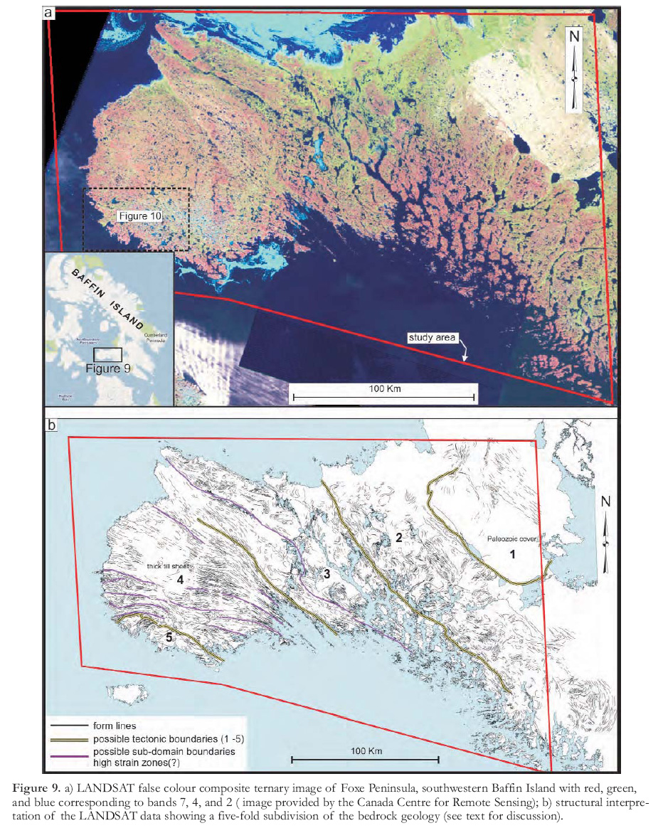
37 Optical imagery can be used to assist in mapping geological structures; for example, lineament mapping on remotely sensed data has long been undertaken by geoscientists (Harris et al. 1987). However, the art of lineament mapping can be taken further by employing simple principles of visual interpretation (especially pattern, shape and context), in concert with field observations (if available), and especially the inspection of magnetic data to add some measure of geological calibration to the lineament interpretation (Fig. 9a, b).
38 Because of lower sun angles, winter imagery offers pseudo 3-D enhancement of terrain features that may be useful for structural interpretations (Fig. 8). Fall imagery is often a preferred choice in boreal forest terrain because of maximum senescence-related differences in vegetation, which can, in turn, enhance some geological structures. However, above the tree line, summer imagery captured in the absence of significant snow cover may be preferred. If LANDSAT data are to be used, particularly if free data are preferred, then the geologist may not have a choice and will have to use what is available on the Canadian Geogratis web site [ http://geogratis.cgdi.gc.ca/].
39 The nature of the bedrock (geological environment) is obviously of particular importance, as much more structural information can usually be extracted from older, complexly deformed rocks than from younger, flat-lying sedimentary rocks (see Fig. 5-11 in Harris and Wickert 2008). The amount of structural information that can be interpreted from optical imagery is also affected by the type, thickness and extent of surficial cover and vegetation, as mentioned previously. The following RPM application in structural interpretation, which developed from the Southwestern Baffin Integrated Geosciences project (St-Onge et al. 2007; Sanborn-Barrie et al. 2008) illustrates the importance of geological environment with respect to the application of optical remote sensing data. A pattern of ductile form lines and folds was derived from an enhanced LANDSAT colour composite image of the Foxe Peninsula (Fig. 9a); two areas with relatively few interpreted structures emerge in the interpretation (Fig. 9b): in the west, a thick layer of glacial till obscures underlying bedrock structures, whereas in the northeast, flat-lying Paleozoic sedimentary rocks offer little structural information (Fig. 9b). The form lines interpreted from LANDSAT data represent tectonic trend lines derived from a variety of structures, including bedding and three generations of foliation. In some cases, the trend lines highlight fold interference patterns, which are expressed as circular to ovoid structures that are also delineated as magnetically variable units on total field and vertical gradient data (not shown). The interpreted trend lines allow southwestern Baffin Island to be divided into five major zones (Fig. 9b). Zone 1 is characterized by an absence of trend information and corresponds to flat-lying Paleozoic (Ordovician) carbonate rocks devoid of mappable structures. Zone 2 comprises magnetically low-relief supracrustal rocks of the Lake Harbour Group, which are intruded by magnetite-bearing plutonic rocks and subsequently folded. Zone 3 represents a corridor of uniformly high magnetic intensity with variable form-patterns comprising ‘straight’ zones and smaller scale folds. Zone 4 is characterized by straight northwest-trending form lines reflecting tectonic modification by a major dextral transcurrent shear zone (Sanborn-Barrie et al. 2008). Zone 5 correlates with supracrustal rocks of the Lona Bay and Schooner Harbour sequences (Sanborn-Barrie et al. 2008) and is characterized by a number of northeast-plunging folds.
40 Close inspection of the LANDSAT data (Fig. 10) reveals that many folds can also be traced on the basis of drainage and topographic patterns (e.g. distribution of bedrock ridges). In fact, correlation between form lines interpreted on the LAND-SAT and magnetic data (not shown) is extremely high, indicating that, in this area, both datasets offer similar information and can act as proxies for each other. Corroboration of remotely predicted ductile structures with structural measurements made in the field highlights the value of LANDSAT for regional geological interpretation. More details on this subject can be found in Harris et al. (2008).
41 Figure 11 shows LANDSAT and ASTER images and associated interpretations for a small area in the southern Foxe Peninsula, Baffin Island. The LANDSAT colour composite image (Fig. 11a) is somewhat blocky in appearance and groups of pixels can be seen. However, the plunging syn-form is clearly visible and form lines can be delineated (Fig. 11c), outlining the local structural setting. LANDSAT has a spatial resolution (pixel size) of 30 m and at scales less than 1:100 000 can be difficult to interpret, although in this case the well-defined synform remains recognizable. The ASTER image (Fig. 11b), which has a resolution of 15 m, provides a clearer rendition of this structure.
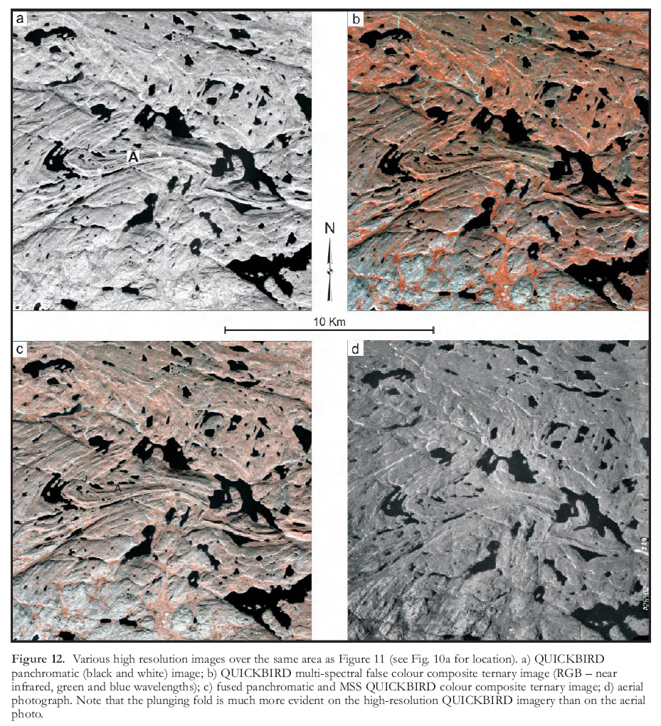
42 Figure 12 presents a series of QUICKBIRD images of the same area as Figure 11. The QUICKBIRD imagery (Fig. 12a to c) provides exceptional structural detail (see Fig. 13b for structural interpretation) exceeding that of an aerial photograph (Fig. 12d). In the higher resolution image (Fig. 12a), a general indication of the northward dip of the southern limb of the syn-form can be ascertained by strong reflections from the scarp slopes facing the sun (south) and less reflection along the dip slopes (see location A on Fig. 12a). The geological structures on the predictive map (Fig. 13b) compare favourably with the mapped geology (St-Onge et al. 2007; Fig. 13a) when comparing form lines and fold axes. However, once again, field work is required to fine tune the predictions and unequivocally identify various geological structures.
 Display large image of Figure 9
 Display large image of Figure 10
 Display large image of Figure 11
Landforms and Glacial Structure
43 Optical imagery can provide useful information on terrain morphology, glacial landforms and streamlined land-forms that reflect glacial dispersal directions (Fig. 14). The degree of topographic/morphologic enhancement will depend on season (see above) and latitude, as variations in both factors will result in different sun elevation and azimuth angles. Combining (fusing) these data with topographic information (i.e. a DEM) often results in a superior image (Fig. 14c) in which glacial landforms are clearly seen. The use of a DEM in conjunction with LANDSAT 7 data for mapping glacial landforms is well illustrated in the Glacial Flow-line Map of Canada (Shaw et al. 2010).
44 Visual photogeologic interpretation of enhanced imagery is commonly undertaken to produce predictive structural maps as shown in Figures 9 to 14. However, automatic and semi-automatic techniques can also be employed to extract linear features (e.g. glacial lineaments), although this approach entails input from the geologist to screen out non-geological lineaments (Masuda et al. 1991; Raghavan et al. 1993; Karnieli et al. 1996).
Bedrock Characterization
45 The Canadian far north has good bedrock exposure, which makes relatively accurate mapping of rock types possible, certainly more so than in boreal forest environments farther south. However, in general, mapping bedrock from optical imagery in northern Canada remains problematic because of surficial and vegetation cover. For example, lichen cover tends to dampen spectral signatures of rocks and sometimes masks important features of individual spectra. Furthermore, optical sensors respond to surface characteristics only, as previously discussed; therefore, spectral signatures often reflect the weathered residue from the underlying bedrock as opposed to the mineral constituents of the rocks themselves. In some cases, this actually facilitates the discrimination of the rocks, which may be distinguished by differences in associated iron and clay weathering products. Many rocks cannot be distinguished solely on the basis of their non-weathered spectral profiles, so this is a viable and valuable approach. In other cases, vegetation cover can be used as a proxy for the underlying bedrock, as certain plant species will grow preferentially over certain rock types, or else the weathered bedrock residue has not been transported by glaciers and therefore reflects, at least in part, the bedrock composition. An approach often utilized before attempting to identify and map rock types from optical data is to mask out areas of surficial and vegetation cover using image-analysis techniques and focusing the analysis on the exposed bedrock or weathered residual material.
 Display large image of Figure 12
 Display large image of Figure 13
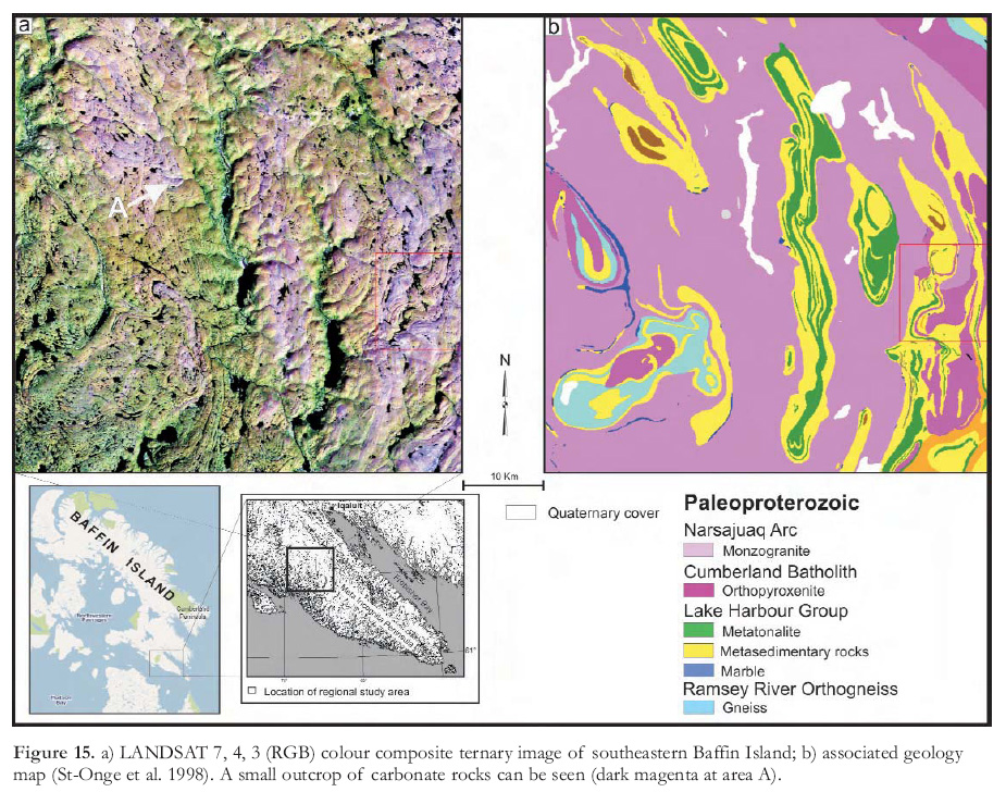
46 Regional differences in litho-types (e.g. basement vs. supracrustal rocks) can often be detected by moderate resolution sensors, such as LAND-SAT, by employing various combinations of bands displayed as colour composite ternary images. On the LANDSAT colour composite image of southeastern Baffin Island (Fig. 15a), note that supracrustal rocks, which define broad doubly plunging folds, are clearly displayed in shades of blue and cyan, whereas basement rocks are displayed in shades of green. Despite the low spectral resolution of LANDSAT data, these rock units are very distinct from a spectral point of view, allowing regional mapping of major rock units and fold patterns. LANDSAT data are especially useful for mapping carbonate-bearing rocks because of their unique signature (even at low spectral resolutions) in the SWIR portion of the EM spectrum (Fig. 15a).
47 Higher spatial and spectral resolution sensors (including hyperspectral) can obviously offer more detailed information on rock types, simply as a function of increased resolution. ASTER, for example, offers better spectral resolution in the SWIR than LANDSAT (see Table 2 and Fig. 11b). A number of examples of the use of ASTER for northern mapping are shown in Harris and Wickert (2008).
48 The SPOT-5 data, although characterized by lower spectral resolution than ASTER or LANDSAT, does offer higher spatial resolution (Table 1) and is valuable not only for lithological mapping but also general logistical planning and field traversing (see section on Field Planning and Logistics below). Figure 16 shows various enhanced SPOT-5 images from Cumberland Peninsula, Nunavut, that illustrate the utility of these multispectral data for differentiating basement and supracrustal rocks.
49 The very high spatial and moderate spectral resolution in the VNIR, together with stereo capability, make imagery captured by GeoEye (and other high-resolution optical sensors) ideal for 2-D and 3-D feature extraction and analysis (Fig. 17). For example, a predictive bedrock geology map interpreted from four stereo Geo-Eye map pairs (Fig. 17c) presents much more detailed information than the existing 1:500 000 scale geological map of the area (Fig. 17d; Thorsteinsson and Tozer 1962; Hulbert et al. 2005). Aided by recent reconnaissance-level field observations, one of the main map units (Wynniatt Formation) was divided into four sub-units (members) that are recognized throughout most of the map area. As well, an important distinction can be made between Proterozoic sedimentary strata and unconformably overlying inter-layered sandstones and carbonates of Cambro-Ordovician age. GeoEye colour composite images provide valuable information about structural and lithological features, and are an excellent resource for bedrock mapping in areas not covered by surficial material (Fig. 18).
 Display large image of Figure 14
50 Hyperspectral remote sensors offer significant advantages over more traditional optical remote sensors (LANDSAT and SPOT) for geological mapping. Increased spectral resolution allows for actual identification of specific minerals (Figs. 5 and 6) and rock types, as opposed to simple discrimination. The main focus of hyperspectral research for geological applications has been the identification of specific minerals, pure concentrations of which are referred to as spectral end members. However, the Arctic, because of the numerous factors discussed above, may represent an environment in which pure end members that relate to specific minerals are difficult, if not impossible, to obtain. Nevertheless, it may be possible to obtain spectral signatures of minerals that typically occur in a certain rock or formation, and to isolate differences in spectra related to the presence or absence of a specific mineral (e.g. Fe- and clay-bearing minerals). Significant research in desert areas of the world has shown that a wide range of minerals, particularly clays, hydroxyl group minerals and carbonates, can be uniquely identified and mapped through spectral analysis (see van der Meer and de Jong 2001) within the VNIR and SWIR regions of the EM spectrum. Much less research has been conducted in cold desert environments typical of Canada’s north. However, recent work, using airborne hyperspectral (PROBE) data in the Canadian Arctic, indicates that dolostones can be uniquely separated from limestones (Budkewitsch et al. 2000) and that metasedimentary, metatonalitic and metagabbroic rocks can be discriminated in certain geological environments (Harris et al. 2005; 2006a, b; 2010). A study by Bowers and Rowen (1996), using hyperspectral data acquired by the Jet Propulsion Laboratory’s AVRIS sensor over the Ice River alkaline complex of British Columbia, also indicated that several bedrock types could be discriminated and identified.
 Display large image of Figure 15
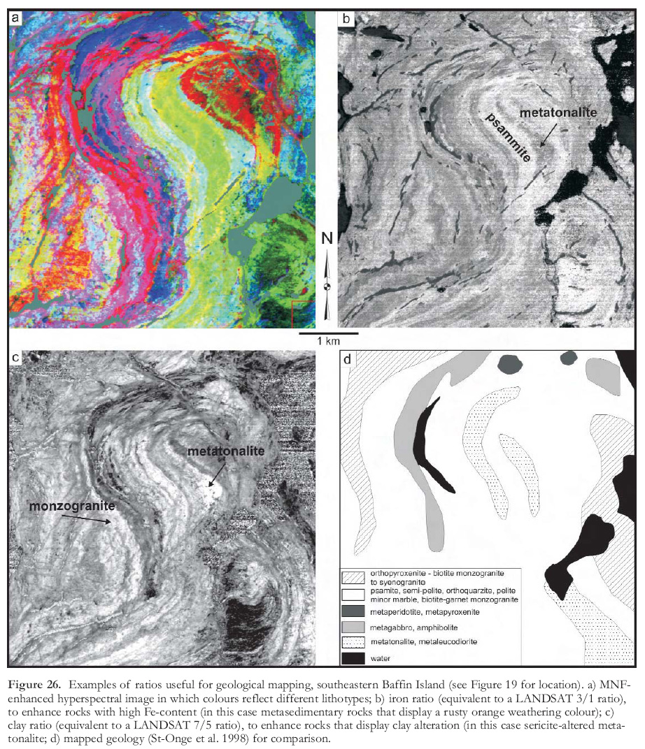
51 Figure 19 is an enhanced hyperspectral image derived from airborne PROBE data acquired over southeastern Baffin Island during August 2000. The various colours on the enhanced image correlate with different rock units, and dark blue areas represent vegetation that grows preferentially over metagabbroic rocks (the vegetation in this area can therefore be used as a mapping proxy). The hyper-spectral imagery was enhanced using a Minimum Noise Fraction transform, a technique for reducing the number of channels (in this case 128) to a smaller number that contains most of the information content of the entire dataset. Harris et al. (2005) provide more details on how this airborne hyperspectral dataset was useful for lithological mapping in southeastern Baffin Island.
52 Lichen cover can be problematic, as it tends to dampen spectral signatures of rocks (Fig. 20) and sometimes masks important features of individual spectra, as previously stated. Again, hyperspectral sensors respond to surface characteristics only; therefore, spectral signatures often reflect the weathered residue from the underlying bedrock as opposed to the mineral constituents of the rocks themselves. It is well known that iron-bearing, hydroxyl-bearing (i.e. clays) and carbonate-bearing rocks are the most easily identified in the VNIR and SWIR because of diagnostic spectral features caused by electronic transitions and molecular vibrations (Hunt 1977; Clarke 1999). Quartzite is also easily identified in the VNIR and SWIR, not because of diagnostic spectral features but because of its high albedo and thus high reflectance. Studies in northern Baffin Island (Budkewitsch et al. 2000) and southeastern Baffin Island (Harris et al. 2005; Rogge et al. 2007, 2009) demonstrate the value of hyper-spectral data for identifying various species of carbonate-bearing rocks, in particular. Figure 21 is a predictive carbonate-image map that combines cal-cite, dolomite, and diopside abundance maps to identify different carbonate species on the basis of subtle differences in spectral reflectance in the SWIR portion of the EM spectrum.
 Display large image of Figure 16
 Display large image of Figure 17
 Display large image of Figure 18
53 For the most part, silicate-bearing rocks do not have diagnostic spectral signatures in the VNIR and SWIR. Thermal remote sensing utilizing emitted radiation in the 8.0 to 14.0 µm range (much longer wavelengths) may be better for mapping silicate-bearing rock types, as it is in this part of the EM spectrum that silicates have unique absorption features.
Surficial Materials
54 Aerial photographs have traditionally been used for surficial mapping through monoscopic and stereoscopic analysis. However, many optical remote sensors now provide spatial resolution comparable to, and, in some cases, exceeding that of aerial photographs. Paired with additional spectral resolution (primarily in the VNIR portion of the EM spectrum) and the ability to collect stereo imagery, new optical sensors provide an excellent source of data to aid in the mapping of Quaternary geology.
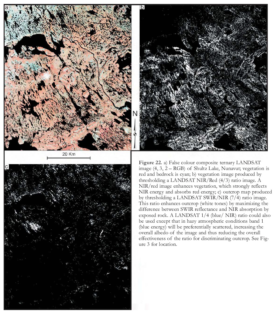
55 Vegetation and wetlands can be easily identified on optical imagery (Fig. 22b), as can bedrock outcrops (Fig. 22c) in most cases, although the spectral signatures of outcrop can be confused with exposed eskers or other glacial features. Various image analysis methods for outcrop identification can be employed, ranging from empirical ratios to supervised classification (Harris and Wickert 2008; also see image examples below). In addition, the location of former forest fires can be identified, which may reveal areas where the probability of outcrop is higher, thus facilitating field traversing.
56 Surficial materials can often be recognized and mapped on enhanced optical imagery through simple visual interpretation based on tones/colour, shape, form, and texture, as well as through more advanced image processing techniques (see below; Grunsky et al. 2006). These predictive maps often compare favourably to mapped surficial units, and depending on the scale, can sometimes offer more information about surficial units than shown on traditional maps (Fig. 23). It should be noted that surficial materials maps can commonly be produced using simple visual interpretation and/or more advanced processing methods, but that maps of glacial processes are more difficult to generate as this involves capturing information other than spectral response.
 Display large image of Figure 19
Field Planning and Logistics
57 Optical imagery can also be used to help in field planning and logistics, although spatial resolution may be a limitation when compared to traditional aerial photographs. However, with the development of sensors that have extremely high spatial resolution from space (e.g. IKONOS, QUICKBIRD, Worldview), logistical planning, aided by satellite-acquired data, is now possible. The major limitation with this type of imagery is the generally higher cost when compared to the purchase of existing aerial photographs, although, as discussed above, they offer comparable or better spatial resolution and certainly better spectral resolution than aerial photos.
58 Optical imagery is frequently an important addition to the new digital technologies being used to conduct field work. Handheld GPS-enabled computer devices are now typically used for recording field observations and are usually equipped with viewing screens that support the display of imagery, including high resolution datasets. This allows for real time display of the geologist’s coordinates on an image dataset, which greatly facilitates traverse navigation. Traditionally, navigation for field work was dependent on having physical copies of black and white aerial photographs; however, the latter can be cumbersome to carry and the photography commonly predates the field visit by many years, resulting in an inaccurate match to the modern landscape. Although the bedrock geology will not change much over time, there may be substantial changes in landforms, extent of surficial materials, and ice cover. Optical imagery is typically much more closely timed to the field visit, e.g. the previous summer. High-resolution imagery commonly exceeds the detail provided in aerial photographs (Fig. 24), and many products have the added benefit of multiple image bands that provide more information on spectral response, thus assisting in mapping various geological features. In addition to the digital displays, paper plots of optical imagery help with helicopter navigation, and allow the geologist to make notes and rough interpretations that can be tested while in the field. Furthermore, optical imagery is by definition digital, whereas most aerial photography is analogue imagery requiring scanning and georeferencing before the data can be used within a GIS environment.
 Display large image of Figure 20
DATA PROCESSING
Visual Enhancement
59 Contrast enhancement involves using a mathematical function (look-up-table or LUT) to stretch the raw data expressed in bytes to the full display range of the data histogram (0–255 grey levels), thus improving the contrast and colour distribution of the image. Figure 25a is a raw image prior to application of a linear LUT, whereas Figure 25b shows the results after contrast stretching.
60 Spatial filtering (edge enhancement and high frequency enhancement) techniques are useful for highlighting geological structures (Fig. 25c, d). Spatial filtering involves the application of a filter to the image data on a pixel-by-pixel basis, either in the image (convolution) or frequency (Fourier) domain, and is used to enhance either low or high spatial frequency features as well as edges in optical imagery. These features often represent geological structures (faults, dykes, form lines, lithological contacts) as well as glacial features (eskers, drumlins, flow features). Note the spatial enhancement of northwest–southeast trending glacial features and northeast–southwest trending tectonic features (Fig. 25c, d) compared to the raw and contrast-stretched images (Fig. 25a, b, respectively).
61 Colour composite ternary images offer significant advantages over single-channel black and white displays for geological interpretation as they combine three channels of often complementary information, resulting in a better portrayal of geological features than when a single channel is used (compare and contrast the single-band black and white images (Fig. 2) with the colour ternary images shown in Fig. 3). Some of the common colour combinations of LANDSAT data used for geological interpretation in northern environments are listed in Table 4.
62 Band ratios (dividing one band by another) are extremely useful for highlighting spectral differences (e.g. reflection vs. absorption) between various surface features, such as vegetation and outcrop (Fig. 22), and iron- and clay-bearing rocks (Fig. 26b, c). Band ratio images can be used to highlight or identify these geological features for further spectral and spatial analysis, or as masks that are used to exclude areas from further processing and analysis (Fig. 16c).
 Display large image of Figure 21
Multivariate Processing
63 Optical multispectral imagery such as LANDSAT is amenable to multivariate processing. A number of data transformations (e.g. Principle Component Analysis and Minimum Noise Fraction; Richards and Jia 1999; Jensen 2005) can be applied to optical data (Figs. 16d, 19) and serve as valuable image processing techniques whereby spectral variations, which often represent differences in lithology and surficial materials, are enhanced. Principal Component Analysis describes the distribution of multivariate data using a new set of transformed axes (components) that are linear combinations of all the input bands. Each component represents a mix of the input bands (the influence of each band is measured by an eigenvector), and can be displayed as an individual black and white image, or else three components can be displayed as an RGB colour composite ternary image (see Fig. 5-28 of Harris and Wickert 2008). The resulting component images can enhance individual features of the terrain, such as vegetation, moisture regimes, rock and surficial units. The Minimum Noise Fraction transformation, examples of which have been presented above, is very similar to Principle Component Analysis except that it is more effective for isolating noise in a multivariate dataset (Green et al. 1988) and is commonly applied to hyperspectral data. Variations of Principal Component Analysis, such as Directed Principal Component Analysis (e.g. Crosta technique; Crosta and Moore 1989), allow for the identification of selected wavelengths that contain spectral information on specific minerals, and the use of these selected wavelengths to perform a Principal Component Analysis. Further details on the use of these multivariate transforms can be found in Grunsky et al. (2006) and Harris and Wickert (2008).
 Display large image of Figure 22
Data Visualization
2.5-D Renditions
64 Geologists have long been using technology to view landscapes in the third dimension to facilitate geological interpretation. In the past, this typically consisted of viewing overlapping aerial photographs through stereoscopes. However, new computer technology and software now provide geologists with a digital environment for viewing multiple image representations of a landscape. The GIS and data visualisation software is now available that enables the use of a DEM (or some other statistical surface data such as magnetics) to build digital 2.5-D terrains that can accommodate the draping of both image and vector data and support the creation of pseudo real-world scenes. Working within these 2.5-D digital environments can assist with visual interpretation of map and image analysis products by highlighting textural information that is not as easily perceived in a planimetric view of the data (Fig. 27a). It can also be useful for logistical planning exercises such as locating suitable sites for field camps and strategically planning field traverses (Fig. 27b).
 Display large image of Figure 23
 Display large image of Table 4
Data Fusion
65 Data fusion (Harris et al. 1990, 1999) is now a standard visualization technique for combining various geoscience datasets. Fusion is accomplished by using a number of image processing techniques (colour space transforms, arithmetic operators, wavelet transforms), the aim of which is to produce an enhanced image suitable for visual interpretation in which elements of the fused data complement one another. Fused imagery provides an image which is greater than the sum of its individual inputs. For example, LANDSAT can be fused with digital elevation data (i.e. a DEM), offering an image that shows spectral patterns through variations in hue, combined with enhanced topography that is useful for highlighting geomorphic patterns (Figs. 12c and 14c). The DEM may also be used to construct a 2.5-D visualization of the terrain (Fig. 27a, b). LANDSAT data may also be fused with thematic data (such as a geological map) so that the geology can be directly compared to the spectral patterns seen on the LANDSAT imagery, or merged with geophysical data so that magnetic patterns can be compared to topographic and spectral patterns. Harris et al. (1990, 1999) provide many examples of effective data fusions for geological interpretation.
 Display large image of Figure 24
Computer Assisted Processing
Supervised Classification
66 A spectral map is based on variations in spectral signatures extracted from optical imagery; geological calibration of these spectral classes must be undertaken by field work or comparison with other supporting geoscience datasets. A spectral map can be created from optical imagery by using a priori information on rock or surficial units, which can take the form of training areas over known rock or surficial units and can be derived by a number of methods, including:
- Inspection of aerial photographs or high resolution satellite imagery;
- Field observations or locations chosen in the field; and
- Inspection of geological maps in concert with observations of optical imagery.
67 Once the geologist has selected suitable training areas that are considered representative of the rock units to be classified, spectral signatures (statistics) for those units are extracted and compared to one another using a variety of statistical techniques (e.g. Transformed Divergence ) to test if the signatures are statistically separable, for each unit to be mapped. If the signatures are unique, statistics from each training area are then used to classify the data by employing a classification algorithm (e.g. Maximum Likelihood; Neural Networks, etc.; see Jensen 2005), resulting in a classified (predictive) map of geological units (Fig. 23; Grunsky et al. 2006). It is often prudent to divide the original training areas into two (or more) groups for cross-validation purposes. That is, one group of training areas can be used for classification and the other group used to validate the classification through what is called a Confusion Matrix. Another method for validating the accuracy of the classification is to compare the classified map to sites visited in the field. Harris et al. (in press) present a new method of supervised classification based on a Monte Carlo simulation (a class of computational algorithms that rely on repeated random sampling to compute their results) in concert with random cross-validation of the training areas used for classifying surficial materials. This algorithm, known as the Iterative Classification method, has the advantage of quantifying both statistical and spatial uncertainty in the classification process.
 Display large image of Figure 25
 Display large image of Figure 26
68 Classification of optical imagery is often only based on spectral information, but optical imagery also potentially offers much textural information that can be used in the classification process in concert with spectral (tonal) information (note: texture is defined as rapid changes in tonal response in an image and defines spatial patterns that are a mix of different spatial frequencies). The addition of spatial derivatives calculated from the optical data and/or other datasets like DEMs and radar can provide additional surface information that often results in higher classification accuracies.
Unsupervised Classification
69 A spectral map can also be produced automatically without input from training areas by using a process known as Unsupervised Classification or Data Clustering. Typically, the geologist will provide the number of units (or clusters) to be found in the multi-band optical data and select a clustering algorithm (e.g. K-means, N-D histogram, etc.) that will automatically find like statistical data clusters and produce a thematic map of these clusters. However, the geologist must make geological sense of this map to determine what the resulting units represent. This normally involves ‘ground truthing’ (field mapping) and/or examination of other supporting geoscience datasets to geologically calibrate the spectral classes. An example of a surficial materials map produced through unsupervised classification is shown in Figure 5-32 of Harris and Wickert (2008).
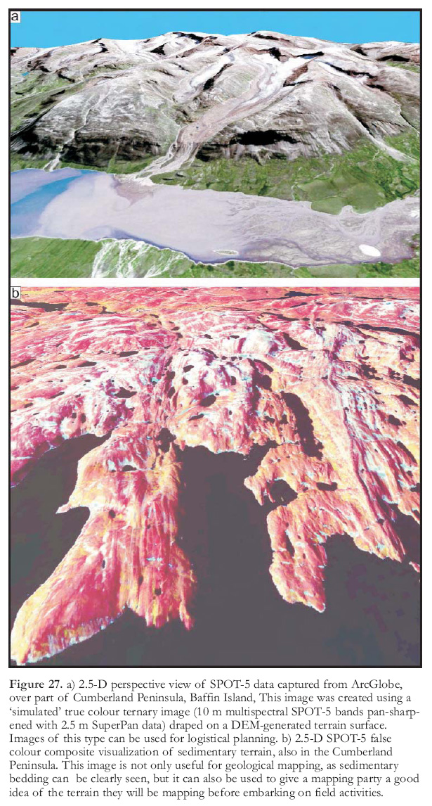 Display large image of Figure 27
DISCUSSION and SUMMARY
70 Optical remote sensing involving the spectral analysis of minerals, rocks and surficial materials plays an important part in the remote predictive mapping process, both for mapping and for exploration activities. The recent emphasis on sensors that offer higher spatial and spectral resolution facilitates the geological mapping and exploration process by providing increased spatial detail, often surpassing that which can be achieved from aerial photographs; it also allows for the unique identification of specific minerals and, in some cases, rock types, based on spectral response (unique spectral characteristics). Discrimination and general separation of certain minerals, rocks and surficial materials are possible with lower spectral resolution sensors (LANDSAT, SPOT), but unique identification, as is the case with hyperspectral sensors, is not.
71 A great variety of optical sensors is presently available, with more coming on line in the near future (e.g. LANDSAT 8, hyperspectral). Most of these will collect data in the VNIR and SWIR segments of the EM spectrum. Much research on the geological applications of remotely sensed data collected in these portions of the EM spectrum exist in the literature, but further research is required on spectral analysis for northern geological environments (especially the application of hyperspectral imagery). An exciting new field, still in its infancy, is the application of thermal remote sensing for the identification of silicate-bearing rocks. However, few satellite-borne sensors other than ASTER offer sufficient spectral resolution for this type of geological application, and the 90 m spatial resolution of ASTER thermal data limits results to a regional scale, at best. At this stage we are still reliant on airborne sensors as we are for hyper-spectral optical remote sensing.
72 Particularly important to the application of optical remote sensing for geological mapping is the nature of the bedrock, including the weathering style of specific rock types, which depends on their mineralogy, the nature and type of surficial cover, geomorphic/topographic characteristics, and biophysical cover (i.e. vegetation and lichens). This, combined with the scale of mapping, not only dictates the choice of a particular optical sensor but also the type of processing required for extracting geological information. Simple image enhancement followed by visual (onscreen) interpretation of 2-D imagery is often very effective, mimicking the procedure long applied by geologists to aerial photographs. It is also now possible to view stereo imagery on touch-sensitive CRT screens using special stereo glasses and to actually conduct photogeo-logic interpretations using touch-sensitive pens, the results of which can be immediately captured as vector files within a GIS environment. The role of more advanced computer processing techniques, especially when dealing with many image channels (e.g. multi-spectral, hyperspectral) offers advantages for producing more objective maps based on the spectral (and textural) characteristics of the data itself. A predictive geological map is often produced using both processing methods.
73 Figure 28 illustrates areas of northern Canada where optical remote sensing is likely to be successful for bedrock and surficial mapping. These maps are derived from the merging (in a GIS platform) of the new International Polar Year compilation of Arctic geology (Harrison et al. 2008), the surficial geology map of Canada (Fulton 1995) and a Canadian landcover map (NRCAN 1999). The areas optimum for bedrock mapping using optical remotely sensed data (Fig. 28a) were ranked following GIS analysis of major rock types and surficial cover. Specifically, rock types that are best separated using spectral analysis (largely sedimentary or supracrustal rocks as opposed to granitoid rocks) and areas that are either exposed or covered with thin till were rated as having higher potential; areas covered by ice obviously have low potential. With respect to structural mapping, older, Archean bedrock generally offers better potential for structural mapping using optical remote sensing than flat-lying sedimentary sequences, especially if geological structures are topographically expressed and not covered by thick till deposits. With respect to the potential for mapping surficial deposits (Fig. 28b), areas of thicker till cover were rated as having lower potential for mapping both materials and landforms, as opposed to less covered areas where landforms, and in some cases surface materials, are strongly expressed in the geomorphic/topographic environment.
74 It is recommended that these maps be used only as a general guide to the selection of optical data for geological mapping. In combination with these maps, a cursory interpretation of LANDSAT data (free from the Geogratis website) would be beneficial to a planned mapping project. As can be seen in the examples provided herein, certain geological environments are more suitable for optical remote sensing of bedrock and geological structures. For example, because of its overall optical spectral properties, Victoria Island (Figs. 17 and 18) is better suited for geological mapping than Baffin Island, and within Baffin Island, mapping supracrustal rocks (Figs. 15 and 19) is more easily done by optical remote sensing in the southeast than in the southwest (Figs. 9 to 13) because of generally less vegetation and lichen cover in the former and the weathering style of the various rock types. From a structural mapping perspective, both environments offer much information, as form lines are well-expressed topo-graphically (e.g. see Figs. 9 and 13). If the LANDSAT data appear promising after examination of the range of colours and patterns seen in the imagery (Figures 9 and 15 provide examples of good spectral contrast), then progression to other, higher resolution data is warranted. However, if the area is well-covered and appears spectrally homogeneous, then another method (e.g. geophysics, radiometrics, radar) may offer more geological information and thus a better source on which to base geological predictions.
75 Optical remote sensing does play, and will play an increasingly important role in the geological mapping of Canada’s north. This is especially relevant with the recent emphasis on satellite-borne systems that offer high spatial and spectral resolutions along with the ability to collect data in stereo, which is obviously advantageous for geological interpretation. The incorporation of optical remote sensing in the development of RPM methods and protocols is presently being undertaken by the Geological Survey of Canada.
 Display large image of Figure 28
We would like to thank Bill Morris and an anonymous reviewer for comments and suggestions that have led to a much improved manuscript. This work was supported by the NRCAN Geo-mapping for Energy and Minerals (GEMS) program under the Remote Predictive Mapping (RPM) project. We would also thank and acknowledge the Geological Association of Canada for publishing this article and the expert editing of Reg Wilson. This represents GSC contribution 20110103.